Take-home Exercise 1: Singapore Private Residential Property Market for 2024 Q1

Author

Kristine Joy Paas

Published

April 16, 2024

Modified

April 26, 2024

1 Overview

1.1 Background

Singapore has one of the highest home ownership rates in the world at 89.7%, 2nd only to Russia among the G20 countries. Due to Singapore’s successful public housing program, 77.8% of Singapore residents live in HDB flats, while 22% live in private properties like condos or landed properties.

While the HDB market targets Singaporeans with household income of up to 14,000 SGD, the private housing market is Singapore is still in demand for households looking to upgrade, invest their property, and for residents not eligible for public housing (e.g. high income household, foreigners, etc.)

In this exercise we will look at the market trends for private residential property market for 2024 Q1 and see how the economic factors have affected it.

1.2 Loading the data sources

For this exercise, we will use the residential real estate transaction data from REALIS. This provides comprehensive and up-to-date statistics on the private property market in Singapore.

The dataset has been provided via eLearn and added to the data/ folder of this exercise.

File Structure

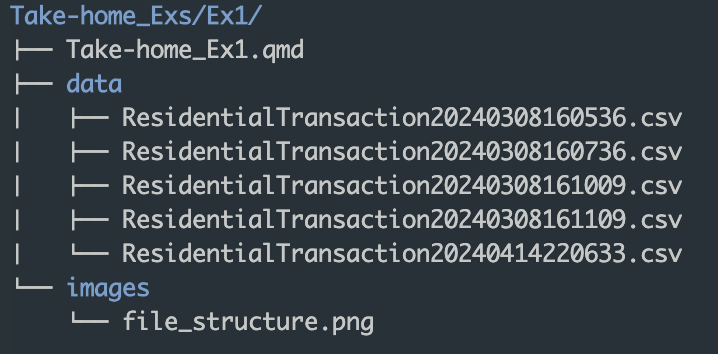
For the purposes of this exercise, we will refer to each data as the following:

2023Q1: ResidentialTransaction20240308160536.csv
2023Q2: ResidentialTransaction20240308160736.csv
2023Q3: ResidentialTransaction20240308161009.csv
2023Q4: ResidentialTransaction20240308161109.csv
2024Q1: ResidentialTransaction20240414220633.csv

1.3 Methodology

To start the data analysis, we first need to prepare the R environment for analysis. This includes loading the R packages and loading the datasets.

After the setup, we need to do data wrangling where we clean and transform the data into a form that is fitting for our analysis. This will possible entail removing irrelevant data, deriving additional variables, renaming columns, etc.

As part of wrangling, we need to decide on what data we would like to look at closely. For the purposes of this exercise, these are the data we can look at that can potentially give valuable insights:

Total units sold by quarter
Units sold by submarkets such as property type (e.g. condominium, terrace house, apartment, detached house), sale type (e.g. resale, new sale, subsale), etc.
Transaction price by submarkets such property type (e.g. condominium, terrace house, apartment, detached house, etc), sale type (e.g. resale, new sale, subsale), etc.

Finally, we will do data exploration and visualize the insights gained from the data. Some of the questions we would ask are:

What is the general trend of private residential property sales prices?
Is this trend consistent among all submarkets?
How affordable are private residential properties for Singaporean households?

2 Setup

2.1 Loading the R packages

For this exercise, we will mainly use the following packages for data analysis:

tidyverse: A collection of R packages used in data science, which includes ggplot2, tibble, readr, among others
ggdist: Provides functions for presenting distributions in ggplot2. stat_halfeye() and stat_dots() will be used the most.
ggtext: Enhances text rendering for ggplot2. element_markdown() is most notable function used for markdown rendering so we can highlight important information in text.
ggrepel: Manages overlapping texts and labels on ggplot2. We will use this to render labels on dense plots.
patchwork: Allows composition of multiple graphs into a single plot

Aside from these, we will also include other packages that will help us present the data better.

knitr: Provides tools for dynamic report generation in R. For this exercise, we will use this package to render our tables better.
scales: Extends functions to operate on ggplot2 scales. For this exercise, we will use wrap_format() to wrap long texts.

pacman::p_load(knitr,
               tidyverse,
               patchwork,
               ggdist,
               ggtext,
               ggrepel,
               scales)

2.2 Data Checkpoints

As the analysis is expected to have a lot of intermediate steps, Save, Load, and Data clear points are available to make our data wrangling more efficient.

Save point

This is where data is written as rds files using write_rds() for important data sets that will be used in later analysis. Examples are:

Data we need to prepare for analysis
Critical outputs of expensive calculations
Cleaned up data for lightweight processing

Load point

This is where data is loaded from rds files using read_rds(). They were previously generated by the save point.

TIP: Skip to the load points to progress without running the code above it

Data clear point

This is where data that will not be used anymore are cleared. The data in RStudio environment will pile up and will make it more difficult to check the relevant data in each part.

We can set #| eval: false in code chunks if we want skip the clearing. For example, the code below won’t be run.

message <- "This code chunk executed"

To use these checkpoints, we need to create data/rds folder.

3 Data Wrangling

3.1 Importing the datasets

Upon inspection of the csv files, column names have human-readable titles such as “Project Name”, “Transacted Price ($)”, etc. While good for humans, these column names may cause parsing issues with R, especially as there are special characters.

Because of this, we will rename the columns in their UPPER_CASE format after removing the special characters. We will create a helper function that will help us accomplish this:

rename_realis_column <- function(orig_name) {
  # Add underscores to spaces
  gsub(" +", "_",
       # Remove special characters
       gsub("[^A-Z ]", "",
            # Convert to upper case and remove trailing spaces
            toupper(orig_name)) %>% trimws())
}

We will use read_csv() to import each file and use rename_realis_column() in the rename_with() function.

realis_2023q1 <- read_csv('data/ResidentialTransaction20240308160536.csv') %>%
                  rename_with(rename_realis_column)
kable(head(realis_2023q1, n=7))

PROJECT_NAME	TRANSACTED_PRICE	AREA_SQFT	UNIT_PRICE_PSF	SALE_DATE	ADDRESS	TYPE_OF_SALE	TYPE_OF_AREA	AREA_SQM	UNIT_PRICE_PSM	NETT_PRICE	PROPERTY_TYPE	NUMBER_OF_UNITS	TENURE	COMPLETION_DATE	PURCHASER_ADDRESS_INDICATOR	POSTAL_CODE	POSTAL_DISTRICT	POSTAL_SECTOR	PLANNING_REGION	PLANNING_AREA
THE REEF AT KING’S DOCK	2317000	882.65	2625	01 Jan 2023	12 HARBOURFRONT AVENUE #05-32	New Sale	Strata	82.0	28256	-	Condominium	1	99 yrs from 12/01/2021	Uncompleted	HDB	097996	04	09	Central Region	Bukit Merah
URBAN TREASURES	1823500	882.65	2066	02 Jan 2023	205 JALAN EUNOS #08-02	New Sale	Strata	82.0	22238	-	Condominium	1	Freehold	Uncompleted	Private	419535	14	41	East Region	Bedok
NORTH GAIA	1421112	1076.40	1320	02 Jan 2023	29 YISHUN CLOSE #08-10	New Sale	Strata	100.0	14211	-	Executive Condominium	1	99 yrs from 15/02/2021	Uncompleted	HDB	269343	27	26	North Region	Yishun
NORTH GAIA	1258112	1033.34	1218	02 Jan 2023	45 YISHUN CLOSE #07-42	New Sale	Strata	96.0	13105	-	Executive Condominium	1	99 yrs from 15/02/2021	Uncompleted	HDB	269294	27	26	North Region	Yishun
PARC BOTANNIA	1280000	871.88	1468	03 Jan 2023	12 FERNVALE STREET #06-16	Resale	Strata	81.0	15802	-	Condominium	1	99 yrs from 28/12/2016	2022	HDB	797391	28	79	North East Region	Sengkang
NANYANG PARK	5870000	3322.85	1767	03 Jan 2023	72 JALAN LIMBOK	Resale	Land	308.7	19015	-	Terrace House	1	999 yrs from 14/02/1881	-	Private	548742	19	54	North East Region	Hougang
PALMS @ SIXTH AVENUE	4950000	4520.88	1095	03 Jan 2023	231 SIXTH AVENUE	Resale	Strata	420.0	11786	-	Semi-Detached House	1	Freehold	2015	Private	275780	10	27	Central Region	Bukit Timah

There are 4,722 private residential propertysales for 2023 Q1.

realis_2023q2 <- read_csv('data/ResidentialTransaction20240308160736.csv') %>%
                  rename_with(rename_realis_column)
kable(head(realis_2023q2, n=7))

PROJECT_NAME	TRANSACTED_PRICE	AREA_SQFT	UNIT_PRICE_PSF	SALE_DATE	ADDRESS	TYPE_OF_SALE	TYPE_OF_AREA	AREA_SQM	UNIT_PRICE_PSM	NETT_PRICE	PROPERTY_TYPE	NUMBER_OF_UNITS	TENURE	COMPLETION_DATE	PURCHASER_ADDRESS_INDICATOR	POSTAL_CODE	POSTAL_DISTRICT	POSTAL_SECTOR	PLANNING_REGION	PLANNING_AREA
THE GAZANIA	1528000	678.13	2253	01 Apr 2023	15 HOW SUN DRIVE #02-31	New Sale	Strata	63	24254	-	Condominium	1	Freehold	2022	N.A	538545	19	53	North East Region	Serangoon
THE GAZANIA	1938000	958.00	2023	01 Apr 2023	7 HOW SUN DRIVE #01-12	New Sale	Strata	89	21775	-	Condominium	1	Freehold	2022	Private	538530	19	53	North East Region	Serangoon
ONE PEARL BANK	2051000	699.66	2931	01 Apr 2023	1 PEARL BANK #32-16	New Sale	Strata	65	31554	-	Apartment	1	99 yrs from 01/03/2019	Uncompleted	Private	169016	03	16	Central Region	Outram
URBAN TREASURES	1850700	882.65	2097	01 Apr 2023	205 JALAN EUNOS #05-05	New Sale	Strata	82	22570	-	Condominium	1	Freehold	Uncompleted	HDB	419535	14	41	East Region	Bedok
HYLL ON HOLLAND	2021500	699.66	2889	01 Apr 2023	97 HOLLAND ROAD #10-25	New Sale	Strata	65	31100	-	Condominium	1	Freehold	Uncompleted	Private	278541	10	27	Central Region	Bukit Timah
LEEDON GREEN	1838000	785.77	2339	01 Apr 2023	34 LEEDON HEIGHTS #12-40	New Sale	Strata	73	25178	-	Condominium	1	Freehold	Uncompleted	Private	266076	10	26	Central Region	Bukit Timah
KLIMT CAIRNHILL	7320000	2055.92	3560	01 Apr 2023	71 CAIRNHILL ROAD #15-01	New Sale	Strata	191	38325	-	Apartment	1	Freehold	Uncompleted	Private	229725	09	22	Central Region	Newton

There are 6,125 private residential property sales for 2023 Q2.

realis_2023q3 <- read_csv('data/ResidentialTransaction20240308161009.csv') %>%
                  rename_with(rename_realis_column)
kable(head(realis_2023q3, n=7))

PROJECT_NAME	TRANSACTED_PRICE	AREA_SQFT	UNIT_PRICE_PSF	SALE_DATE	ADDRESS	TYPE_OF_SALE	TYPE_OF_AREA	AREA_SQM	UNIT_PRICE_PSM	NETT_PRICE	PROPERTY_TYPE	NUMBER_OF_UNITS	TENURE	COMPLETION_DATE	PURCHASER_ADDRESS_INDICATOR	POSTAL_CODE	POSTAL_DISTRICT	POSTAL_SECTOR	PLANNING_REGION	PLANNING_AREA
MYRA	1658000	667.37	2484	01 Jul 2023	9 MEYAPPA CHETTIAR ROAD #02-07	New Sale	Strata	62	26742	-	Apartment	1	Freehold	Uncompleted	N.A	358456	13	35	Central Region	Toa Payoh
NORTH GAIA	1449000	1076.40	1346	01 Jul 2023	27 YISHUN CLOSE #10-06	New Sale	Strata	100	14490	-	Executive Condominium	1	99 yrs from 15/02/2021	Uncompleted	HDB	769342	27	76	North Region	Yishun
NORTH GAIA	1365000	1076.40	1268	01 Jul 2023	27 YISHUN CLOSE #05-06	New Sale	Strata	100	13650	-	Executive Condominium	1	99 yrs from 15/02/2021	Uncompleted	HDB	769342	27	76	North Region	Yishun
NORTH GAIA	1231000	958.00	1285	01 Jul 2023	35 YISHUN CLOSE #08-25	New Sale	Strata	89	13831	-	Executive Condominium	1	99 yrs from 15/02/2021	Uncompleted	HDB	769299	27	76	North Region	Yishun
NORTH GAIA	1272000	1001.05	1271	01 Jul 2023	45 YISHUN CLOSE #09-45	New Sale	Strata	93	13677	-	Executive Condominium	1	99 yrs from 15/02/2021	Uncompleted	HDB	769294	27	76	North Region	Yishun
PICCADILLY GRAND	3462000	1679.18	2062	01 Jul 2023	3 NORTHUMBERLAND ROAD #14-09	New Sale	Strata	156	22192	-	Apartment	1	99 yrs from 02/08/2021	Uncompleted	Private	219569	08	21	Central Region	Kallang
TENET	1356000	925.70	1465	01 Jul 2023	71 TAMPINES STREET 62 #14-02	New Sale	Strata	86	15767	-	Executive Condominium	1	99 yrs from 01/11/2021	Uncompleted	HDB	529699	18	52	East Region	Tampines

There are 6,206 private residential property sales for 2023 Q3.

realis_2023q4 <- read_csv('data/ResidentialTransaction20240308161109.csv') %>%
                  rename_with(rename_realis_column)
kable(head(realis_2023q4, n=7))

PROJECT_NAME	TRANSACTED_PRICE	AREA_SQFT	UNIT_PRICE_PSF	SALE_DATE	ADDRESS	TYPE_OF_SALE	TYPE_OF_AREA	AREA_SQM	UNIT_PRICE_PSM	NETT_PRICE	PROPERTY_TYPE	NUMBER_OF_UNITS	TENURE	COMPLETION_DATE	PURCHASER_ADDRESS_INDICATOR	POSTAL_CODE	POSTAL_DISTRICT	POSTAL_SECTOR	PLANNING_REGION	PLANNING_AREA
LEEDON GREEN	1749000	538.20	3250	01 Oct 2023	26 LEEDON HEIGHTS #11-08	New Sale	Strata	50	34980	-	Condominium	1	Freehold	Uncompleted	Private	266221	10	26	Central Region	Bukit Timah
LIV @ MB	3148740	1453.14	2167	01 Oct 2023	114A ARTHUR ROAD #01-01	New Sale	Strata	135	23324	-	Condominium	1	99 yrs from 23/11/2021	Uncompleted	Private	439826	15	43	Central Region	Marine Parade
MORI	2422337	1259.39	1923	01 Oct 2023	223 GUILLEMARD ROAD #05-21	New Sale	Strata	117	20704	-	Apartment	1	Freehold	Uncompleted	Private	399738	14	39	Central Region	Geylang
THE ARDEN	1330000	721.19	1844	01 Oct 2023	6 PHOENIX ROAD #01-18	New Sale	Strata	67	19851	-	Apartment	1	99 yrs from 14/07/2023	Uncompleted	Private	668159	23	66	West Region	Bukit Batok
LENTOR MODERN	2237000	1130.22	1979	01 Oct 2023	3 LENTOR CENTRAL #05-03	New Sale	Strata	105	21305	-	Apartment	1	99 yrs from 26/10/2021	Uncompleted	Private	788888	26	78	North East Region	Ang Mo Kio
THE LAKEGARDEN RESIDENCES	1249900	592.02	2111	01 Oct 2023	82 YUAN CHING ROAD #04-14	New Sale	Strata	55	22725	-	Condominium	1	99 yrs from 31/05/2023	Uncompleted	HDB	619614	22	61	West Region	Jurong East
LENTOR HILLS RESIDENCES	2890000	1356.26	2131	01 Oct 2023	31 LENTOR HILLS ROAD #15-03	New Sale	Strata	126	22937	-	Apartment	1	99 yrs from 25/04/2022	Uncompleted	HDB	788881	26	78	North East Region	Ang Mo Kio

There are 4,851 private residential property sales for 2023 Q4.

realis_2024q1 <- read_csv('data/ResidentialTransaction20240414220633.csv') %>%
                  rename_with(rename_realis_column)
kable(head(realis_2024q1, n=7))

PROJECT_NAME	TRANSACTED_PRICE	AREA_SQFT	UNIT_PRICE_PSF	SALE_DATE	ADDRESS	TYPE_OF_SALE	TYPE_OF_AREA	AREA_SQM	UNIT_PRICE_PSM	NETT_PRICE	PROPERTY_TYPE	NUMBER_OF_UNITS	TENURE	COMPLETION_DATE	PURCHASER_ADDRESS_INDICATOR	POSTAL_CODE	POSTAL_DISTRICT	POSTAL_SECTOR	PLANNING_REGION	PLANNING_AREA
THE LANDMARK	2726888	1076.40	2533	01 Jan 2024	173 CHIN SWEE ROAD #22-11	New Sale	Strata	100	27269	-	Condominium	1	99 yrs from 28/08/2020	Uncompleted	Private	169878	03	16	Central Region	Outram
POLLEN COLLECTION	3850000	1808.35	2129	01 Jan 2024	34 POLLEN PLACE	New Sale	Land	168	22917	-	Terrace House	1	99 yrs from 09/12/2019	Uncompleted	N.A	807233	28	80	North East Region	Serangoon
SKY EDEN@BEDOK	2346000	1087.16	2158	01 Jan 2024	1 BEDOK CENTRAL #09-10	New Sale	Strata	101	23228	-	Apartment	1	99 yrs from 05/01/2022	Uncompleted	HDB	469657	16	46	East Region	Bedok
TERRA HILL	2190000	807.30	2713	01 Jan 2024	18A YEW SIANG ROAD #03-12	New Sale	Strata	75	29200	-	Apartment	1	Freehold	Uncompleted	N.A	118992	05	11	Central Region	Queenstown
PINETREE HILL	1954000	796.54	2453	01 Jan 2024	36 PINE GROVE #05-18	New Sale	Strata	74	26405	-	Condominium	1	99 yrs from 12/09/2022	Uncompleted	Private	598444	21	59	Central Region	Bukit Timah
THE RESERVE RESIDENCES	3412201	1323.97	2577	01 Jan 2024	13 JALAN ANAK BUKIT #28-106	New Sale	Strata	123	27741	-	Apartment	1	99 yrs from 29/11/2021	Uncompleted	Private	589605	21	58	Central Region	Bukit Timah
SUMMER VILLAS	2960000	3530.59	838	02 Jan 2024	73 GERALD DRIVE #01-06	Resale	Strata	328	9024	-	Terrace House	1	Freehold	2004	Private	797703	28	79	North East Region	Hougang

There are 4,902 private residential property sales for 2024 Q1.

glimpse(realis_2023q1)

Rows: 4,722
Columns: 21
$ PROJECT_NAME                <chr> "THE REEF AT KING'S DOCK", "URBAN TREASURE…
$ TRANSACTED_PRICE            <dbl> 2317000, 1823500, 1421112, 1258112, 128000…
$ AREA_SQFT                   <dbl> 882.65, 882.65, 1076.40, 1033.34, 871.88, …
$ UNIT_PRICE_PSF              <dbl> 2625, 2066, 1320, 1218, 1468, 1767, 1095, …
$ SALE_DATE                   <chr> "01 Jan 2023", "02 Jan 2023", "02 Jan 2023…
$ ADDRESS                     <chr> "12 HARBOURFRONT AVENUE #05-32", "205 JALA…
$ TYPE_OF_SALE                <chr> "New Sale", "New Sale", "New Sale", "New S…
$ TYPE_OF_AREA                <chr> "Strata", "Strata", "Strata", "Strata", "S…
$ AREA_SQM                    <dbl> 82.0, 82.0, 100.0, 96.0, 81.0, 308.7, 420.…
$ UNIT_PRICE_PSM              <dbl> 28256, 22238, 14211, 13105, 15802, 19015, …
$ NETT_PRICE                  <chr> "-", "-", "-", "-", "-", "-", "-", "-", "-…
$ PROPERTY_TYPE               <chr> "Condominium", "Condominium", "Executive C…
$ NUMBER_OF_UNITS             <dbl> 1, 1, 1, 1, 1, 1, 1, 1, 1, 1, 1, 1, 1, 1, …
$ TENURE                      <chr> "99 yrs from 12/01/2021", "Freehold", "99 …
$ COMPLETION_DATE             <chr> "Uncompleted", "Uncompleted", "Uncompleted…
$ PURCHASER_ADDRESS_INDICATOR <chr> "HDB", "Private", "HDB", "HDB", "HDB", "Pr…
$ POSTAL_CODE                 <chr> "097996", "419535", "269343", "269294", "7…
$ POSTAL_DISTRICT             <chr> "04", "14", "27", "27", "28", "19", "10", …
$ POSTAL_SECTOR               <chr> "09", "41", "26", "26", "79", "54", "27", …
$ PLANNING_REGION             <chr> "Central Region", "East Region", "North Re…
$ PLANNING_AREA               <chr> "Bukit Merah", "Bedok", "Yishun", "Yishun"…

The imported dataset has 21 variables.

3.2 Combining the dataframes

Next, we will combine all 5 realis_202*q* dataframes into a single one to simplify aggregation and partitioning of data for analysis.

This will also simplify cleanup and transformation as they will be done on a single dataframe instead of 5.

To do this, we need to add QUARTER values to each dataframe before merging them to a single one. We will use the format <YEAR>Q<QUARTER>, i.e 2024Q1 for 2024 Q1. This is so we can identify which quarter the sale was made, which we will use for aggregation.

Functions used

mutate() for adding new column
rbind() for combining all dataframes
seq_len() and nrow() for generating a sequence of IDs
sprintf() for formatting a string.

realis_2023q1 <- mutate(realis_2023q1, QUARTER="2023Q1")
realis_2023q2 <- mutate(realis_2023q2, QUARTER="2023Q2")
realis_2023q3 <- mutate(realis_2023q3, QUARTER="2023Q3")
realis_2023q4 <- mutate(realis_2023q4, QUARTER="2023Q4")
realis_2024q1 <- mutate(realis_2024q1, QUARTER="2024Q1")

realis <- realis_2023q1 %>%
  rbind(realis_2023q2) %>%
  rbind(realis_2023q3) %>%
  rbind(realis_2023q4) %>%
  rbind(realis_2024q1)
kable(head(realis, n=10))

PROJECT_NAME	TRANSACTED_PRICE	AREA_SQFT	UNIT_PRICE_PSF	SALE_DATE	ADDRESS	TYPE_OF_SALE	TYPE_OF_AREA	AREA_SQM	UNIT_PRICE_PSM	NETT_PRICE	PROPERTY_TYPE	NUMBER_OF_UNITS	TENURE	COMPLETION_DATE	PURCHASER_ADDRESS_INDICATOR	POSTAL_CODE	POSTAL_DISTRICT	POSTAL_SECTOR	PLANNING_REGION	PLANNING_AREA	QUARTER
THE REEF AT KING’S DOCK	2317000	882.65	2625	01 Jan 2023	12 HARBOURFRONT AVENUE #05-32	New Sale	Strata	82.0	28256	-	Condominium	1	99 yrs from 12/01/2021	Uncompleted	HDB	097996	04	09	Central Region	Bukit Merah	2023Q1
URBAN TREASURES	1823500	882.65	2066	02 Jan 2023	205 JALAN EUNOS #08-02	New Sale	Strata	82.0	22238	-	Condominium	1	Freehold	Uncompleted	Private	419535	14	41	East Region	Bedok	2023Q1
NORTH GAIA	1421112	1076.40	1320	02 Jan 2023	29 YISHUN CLOSE #08-10	New Sale	Strata	100.0	14211	-	Executive Condominium	1	99 yrs from 15/02/2021	Uncompleted	HDB	269343	27	26	North Region	Yishun	2023Q1
NORTH GAIA	1258112	1033.34	1218	02 Jan 2023	45 YISHUN CLOSE #07-42	New Sale	Strata	96.0	13105	-	Executive Condominium	1	99 yrs from 15/02/2021	Uncompleted	HDB	269294	27	26	North Region	Yishun	2023Q1
PARC BOTANNIA	1280000	871.88	1468	03 Jan 2023	12 FERNVALE STREET #06-16	Resale	Strata	81.0	15802	-	Condominium	1	99 yrs from 28/12/2016	2022	HDB	797391	28	79	North East Region	Sengkang	2023Q1
NANYANG PARK	5870000	3322.85	1767	03 Jan 2023	72 JALAN LIMBOK	Resale	Land	308.7	19015	-	Terrace House	1	999 yrs from 14/02/1881	-	Private	548742	19	54	North East Region	Hougang	2023Q1
PALMS @ SIXTH AVENUE	4950000	4520.88	1095	03 Jan 2023	231 SIXTH AVENUE	Resale	Strata	420.0	11786	-	Semi-Detached House	1	Freehold	2015	Private	275780	10	27	Central Region	Bukit Timah	2023Q1
N.A.	3260000	1555.40	2096	03 Jan 2023	19 TENG TONG ROAD	Resale	Land	144.5	22561	-	Terrace House	1	Freehold	1941	Private	423510	15	42	Central Region	Marine Parade	2023Q1
WHISTLER GRAND	850000	441.32	1926	03 Jan 2023	107 WEST COAST VALE #30-04	Sub Sale	Strata	41.0	20732	-	Apartment	1	99 yrs from 07/05/2018	2022	HDB	126751	05	12	West Region	Clementi	2023Q1
NORTHOAKS	1268000	1603.84	791	03 Jan 2023	30 WOODLANDS CRESCENT #01-11	Resale	Strata	149.0	8510	-	Executive Condominium	1	99 yrs from 16/12/1997	2000	HDB	738086	25	73	North Region	Woodlands	2023Q1

We will also add TXN_ID so we can more easily refer to the observations later on. The format is TXN00000.

realis$TXN_ID <- sprintf("TXN%05d", seq_len(nrow(realis)))

Let us check if all rows are accounted for by checking if the number of rows in realis is the total number of rows from all dataframes.

nrow(realis) == nrow(realis_2023q1) +
  nrow(realis_2023q2) +
  nrow(realis_2023q3) +
  nrow(realis_2023q4) +
  nrow(realis_2024q1)

[1] TRUE

3.3 Filtering relevant columns

After adding the QUARTER and TXN_ID columns, there are now 23 variables in the dataframe. However, not all of them are relevant to answer the questions we are asking. The table below summarizes the columns and whether we will keep them or not.

Column Name	Description	Reason
TXN_ID	Identifier for the transaction	It is an identifier
QUARTER	Quarter when the property was sold	Core data for aggregation
PROJECT_NAME	Name of the project	Can be used to pinpoint popular projects
TRANSACTED_PRICE	Transaction price (SGD)	Useful for deriving insights
AREA_SQFT	Area of the property in sqft	Useful for deriving insights
UNIT_PRICE_PSF	Price per sqft	Useful for price analysis
TYPE_OF_SALE	One of New Sale, Resale, Subsale	Important submarket information
TYPE_OF_AREA	One of Landed, Strata	Can be used to partition data
PROPERTY_TYPE	Type of Property, e.g. Apartment, Condominium, Executive Condominium, Terrace House, Semi-Detached House, Detached House	Can be used to partition data
NUMBER_OF_UNITS	Number of units involved in the transaction	Core data for analysis
POSTAL_DISTRICT	District where the property is located	Can be used to partition data
TENURE	Can be Freehold or Leasehold	Can be used to partition data

Column Name	Description	Reason
SALE_DATE	Date when the sale was made	We will aggregate by quarter, no need to know the specific dates.
ADDRESS	Property Address	Will use `PROJECT_NAME` if needed to pinpoint projects
AREA_SQM	Price per sqm	`AREA_SFT` is adequate
UNIT_PRICE_PSM	Price per sqm	`UNIT_PRICE_PSF` is adequate
NETT_PRICE		Column is blank
COMPLETION_DATE	When the property was completed. Some properties are Uncompleted as they will be turned over for the future	Other attributes (e.g. `TYPE_OF_SALE`, `PROPERTY_TYPE`) are more important for checking submarket trends
PURCHASER_ADDRESS_INDICATOR	Type of residence of the purchaser	No interest in buyer’s current address
POSTAL_CODE	Postal code of the property	Will use `POSTAL_DISTRICT` for location
POSTAL_SECTOR	Sector where the property is located	Will use `POSTAL_DISTRICT` for location
PLANNING_REGION	Region where the property is located	Will use `POSTAL_DISTRICT` for location
PLANNING_AREA	Area where the property is located	Will use `POSTAL_DISTRICT` for location

We will now use select() to keep only the relevant columns. We will define the function below for filtering the relevant columns. This will also rearrange the columns based on the order in the function call.

realis <-
  realis %>% select(
    c(
      TXN_ID,
      QUARTER,
      PROJECT_NAME,
      TRANSACTED_PRICE,
      AREA_SQFT,
      UNIT_PRICE_PSF,
      TYPE_OF_SALE,
      TYPE_OF_AREA,
      PROPERTY_TYPE,
      NUMBER_OF_UNITS,
      POSTAL_DISTRICT,
      TENURE
    )
  )
glimpse(realis)

Rows: 26,806
Columns: 12
$ TXN_ID           <chr> "TXN00001", "TXN00002", "TXN00003", "TXN00004", "TXN0…
$ QUARTER          <chr> "2023Q1", "2023Q1", "2023Q1", "2023Q1", "2023Q1", "20…
$ PROJECT_NAME     <chr> "THE REEF AT KING'S DOCK", "URBAN TREASURES", "NORTH …
$ TRANSACTED_PRICE <dbl> 2317000, 1823500, 1421112, 1258112, 1280000, 5870000,…
$ AREA_SQFT        <dbl> 882.65, 882.65, 1076.40, 1033.34, 871.88, 3322.85, 45…
$ UNIT_PRICE_PSF   <dbl> 2625, 2066, 1320, 1218, 1468, 1767, 1095, 2096, 1926,…
$ TYPE_OF_SALE     <chr> "New Sale", "New Sale", "New Sale", "New Sale", "Resa…
$ TYPE_OF_AREA     <chr> "Strata", "Strata", "Strata", "Strata", "Strata", "La…
$ PROPERTY_TYPE    <chr> "Condominium", "Condominium", "Executive Condominium"…
$ NUMBER_OF_UNITS  <dbl> 1, 1, 1, 1, 1, 1, 1, 1, 1, 1, 1, 1, 1, 1, 1, 1, 1, 1,…
$ POSTAL_DISTRICT  <chr> "04", "14", "27", "27", "28", "19", "10", "15", "05",…
$ TENURE           <chr> "99 yrs from 12/01/2021", "Freehold", "99 yrs from 15…

After this initial cleanup, we are left with 12 variables relevant to our exploration.

Save point

Let us save realis so we do not need to rerun the steps above.

write_rds(realis, "data/rds/realis_cleaned.rds")

Data clear point

We do not need the realis_202*q* dataframes anymore so we can remove them from the RStudio environment.

rm(realis_2023q1)
rm(realis_2023q2)
rm(realis_2023q3)
rm(realis_2023q4)
rm(realis_2024q1)

3.4 Closer look at NUMBER_OF_UNITS

Load point

We can continue running the document from this point by loading the following prepared data.

realis <- read_rds("data/rds/realis_cleaned.rds")

Taking a closer look at NUMBER_OF_UNITS columns reveals that 12 out of 26,806 transactions involve multiple units.

realis[order(-realis$NUMBER_OF_UNITS),] %>% filter(NUMBER_OF_UNITS > 1) %>% kable()

TXN_ID	QUARTER	PROJECT_NAME	TRANSACTED_PRICE	AREA_SQFT	UNIT_PRICE_PSF	TYPE_OF_SALE	TYPE_OF_AREA	PROPERTY_TYPE	NUMBER_OF_UNITS	POSTAL_DISTRICT	TENURE
TXN01567	2023Q1	MEYER PARK	392180000	144883.44	2707	Resale	Strata	Condominium	60	15	Freehold
TXN00083	2023Q1	BAGNALL COURT	115280000	68491.33	1683	Resale	Strata	Condominium	43	16	Freehold
TXN08370	2023Q2	KEW LODGE	66800000	25177.00	2653	Resale	Strata	Terrace House	11	11	Freehold
TXN17572	2023Q4	KARTAR APARTMENTS	18000000	6964.31	2585	Resale	Strata	Apartment	7	11	Freehold
TXN00861	2023Q1	MONDO MANSION BUILDING	6280000	5489.64	1144	Resale	Strata	Apartment	4	19	Freehold
TXN10593	2023Q2	N.A.	10600000	6746.88	1571	Resale	Strata	Apartment	4	15	Freehold
TXN04100	2023Q1	N.A.	61080008	32148.84	1900	Resale	Land	Detached House	3	11	Freehold
TXN06865	2023Q2	N.A.	32200000	14123.44	2280	Resale	Land	Detached House	2	11	Freehold
TXN10316	2023Q2	N.A.	6150000	4342.20	1416	Resale	Land	Semi-Detached House	2	19	Freehold
TXN12792	2023Q3	EAST VIEW GARDEN	6100000	8337.79	732	Resale	Land	Semi-Detached House	2	16	Freehold
TXN13376	2023Q3	N.A.	8000000	3658.68	2187	Resale	Land	Semi-Detached House	2	14	Freehold
TXN24770	2024Q1	CLAYMORE PLAZA	7000000	4208.72	1663	Resale	Strata	Apartment	2	09	Freehold

Furthermore, the TRANSACTED_PRICE for such transactions are hundred million dollar transactions, which can skew the data if we are looking at TRANSACTED_PRICE with the assumption that it is the price per unit.

For example TXN01567, is worth $392,180,000, which is much higher that the price of individual units

3.5 Handling the bulk transactions

To address the 12 bulk transactions in our dataframe, we have 2 possible options:

Option 1: Remove these transactions as these correspond to 0.045% of transactions (EASY)
Option 2: Create rows for each unit in the transaction (HARD)

Although Option 2 is more difficult, it is the better approach as all the transactions are Resale transactions. Simply removing them may remove very important data for the resale submarket.

For this solution, we need to do the following:

Repeat all rows by NUMBER_OF_UNITS times.
Set transacted price to the average price: $T R A N S A C T E D_P R I C E \div N U M B E R_O F_U N I T S$ .
Set the area (sqft) to the average area: $A R E A_S Q F T \div N U M B E R_O F_U N I T S$ .
Set NUMBER_OF_UNITS to 1.

Repeating rows
Setting column values

Reference: Stackoverflow

Functions used

rep() - to repeat a dataframe

seq_len(nrow()) - to iterate to each row of the dataframe

sales_txns <- realis[rep(seq_len(nrow(realis)), realis$NUMBER_OF_UNITS),]

Lets’ check if the number of rows correspond to the total number of units sold.

nrow(sales_txns) == sum(realis$NUMBER_OF_UNITS)

[1] TRUE

We will perform the changes to NUMBER_OF_UNITS, TRANSACTED_PRICE, AREA_SQFT in 1 code chunk so that rerunning the code chunk is idempotent and won’t mutate the variable further

sales_txns <- sales_txns %>%
  filter(NUMBER_OF_UNITS > 1) %>%
  mutate(TRANSACTED_PRICE = round(TRANSACTED_PRICE / NUMBER_OF_UNITS, 0)) %>%
  mutate(AREA_SQFT = round(AREA_SQFT / NUMBER_OF_UNITS, 0)) %>%
  mutate(NUMBER_OF_UNITS = 1) %>%
  rbind(sales_txns %>% # Reconnect to the rest of the dataframe
              filter(NUMBER_OF_UNITS == 1))

Let us verify the result of the transformation.

Before
After

realis %>%
  filter(TXN_ID %in% c(
    "TXN00001", "TXN00002", # Single-unit transactions
    "TXN10593", "TXN13376" # Bulk transactions
    )) %>% kable()

TXN_ID	QUARTER	PROJECT_NAME	TRANSACTED_PRICE	AREA_SQFT	UNIT_PRICE_PSF	TYPE_OF_SALE	TYPE_OF_AREA	PROPERTY_TYPE	NUMBER_OF_UNITS	POSTAL_DISTRICT	TENURE
TXN00001	2023Q1	THE REEF AT KING’S DOCK	2317000	882.65	2625	New Sale	Strata	Condominium	1	04	99 yrs from 12/01/2021
TXN00002	2023Q1	URBAN TREASURES	1823500	882.65	2066	New Sale	Strata	Condominium	1	14	Freehold
TXN10593	2023Q2	N.A.	10600000	6746.88	1571	Resale	Strata	Apartment	4	15	Freehold
TXN13376	2023Q3	N.A.	8000000	3658.68	2187	Resale	Land	Semi-Detached House	2	14	Freehold

sales_txns %>%
  filter(TXN_ID %in% c(
    "TXN00001", "TXN00002", # Single-unit transactions
    "TXN10593", "TXN13376" # Bulk transactions
    )) %>% kable()

TXN_ID	QUARTER	PROJECT_NAME	TRANSACTED_PRICE	AREA_SQFT	UNIT_PRICE_PSF	TYPE_OF_SALE	TYPE_OF_AREA	PROPERTY_TYPE	NUMBER_OF_UNITS	POSTAL_DISTRICT	TENURE
TXN10593	2023Q2	N.A.	2650000	1687.00	1571	Resale	Strata	Apartment	1	15	Freehold
TXN10593	2023Q2	N.A.	2650000	1687.00	1571	Resale	Strata	Apartment	1	15	Freehold
TXN10593	2023Q2	N.A.	2650000	1687.00	1571	Resale	Strata	Apartment	1	15	Freehold
TXN10593	2023Q2	N.A.	2650000	1687.00	1571	Resale	Strata	Apartment	1	15	Freehold
TXN13376	2023Q3	N.A.	4000000	1829.00	2187	Resale	Land	Semi-Detached House	1	14	Freehold
TXN13376	2023Q3	N.A.	4000000	1829.00	2187	Resale	Land	Semi-Detached House	1	14	Freehold
TXN00001	2023Q1	THE REEF AT KING’S DOCK	2317000	882.65	2625	New Sale	Strata	Condominium	1	04	99 yrs from 12/01/2021
TXN00002	2023Q1	URBAN TREASURES	1823500	882.65	2066	New Sale	Strata	Condominium	1	14	Freehold

Save point

Let us save sales_txns so we do not need to rerun the steps above.

write_rds(sales_txns, "data/rds/sales_txns.rds")

Data clear point

We will use sales_txns from now on so we can remove realis from the environment.

rm(realis)

4 Data Exploration

Load point

We can continue running the document from this point by loading the following prepared data.

sales_txns <- read_rds("data/rds/sales_txns.rds")

4.1 Defining the audience and purpose of the visualizations

4.1.1 Considerations

It is important to note that it is quite challenging to present all data available with just 3 visualizations. We cannot cover all ground and visualize the data from all perspectives, and some blind spots and biases are bound occur in the process.

With this in mind, it is important that we define the audience and purpose of the visualizations.

The audience is a prospective private property buyer that needs help answering these questions in making decisions on buying property:

Should I buy a new property or a resale property?
Should I buy a condo, apartment, or is it worth it to save more for a landed property?
Which districts should I consider when buying a property?
Do I get a bargain compared to buying a property last year?

To answer the questions above, we will focus on exploring and visualizing the distribution among the different markets (New Sale, Resale, Sub Sale).

The points of interest are:

Prices (unit and total)
Distribution across different markets
Distribution by property type

Risks when selecting data to present

As we have limited space to present data (within 2-3 visualizations), we cannot include all the data available to us.

With this, some perspectives may be missed and we will not be able to dive deep enough all aspects of the data.

4.1.2 Unit Price vs Transacted Price

Given AREA_SQFT and UNIT_PRICE_PSF, it is intuitive to expect that: $A R E A_S Q F T \times U N I T_P R I C E_P S F = T R A N S A C T E D_P R I C E$

However, there are only 7 out of 26,936 transactions for which this is true.

sales_txns %>% filter(TRANSACTED_PRICE == AREA_SQFT * UNIT_PRICE_PSF) %>% nrow()

[1] 7

This is because the final transacted price depends on other factors like size of property, floor height, where the property is facing, etc. Most of these factors are not reflected in the dataset we have.

Hence, to have a fairer comparison with what we have, we will use UNIT_PRICE_PSF for price comparisons.

4.1.3 Compare all quarters or two quarters

In answering the questions we define (and based on the specifications of the exercise), the data partition for the visualization is by TYPE_OF_SALE as we want to look for trends from the different submarkets.

We current have 5 quarters in our dataset, 3 submarkets. This means 15 facets, which may be too much for division for visualization. It is also difficult to see at a glance when information we are trying to communicate if there are many very small graphs.

In addition, if we want to dive even deeper by PROPERTY_TYPE, which has 6 possible values, that is 90 data subsets we need to present.

Hence to simplify the visualization, we will choose only the 2023Q1 and 2024Q1, which should suffice for our purpose of comparing the state of the market to last year’s as we are comparing the same time of the year.

Hence, we will produce the data frames to contain these data.

sales_txns_q1_2324 <- sales_txns %>% filter(QUARTER %in% c("2023Q1", "2024Q1"))
sales_txns_q1_23 <- sales_txns_q1_2324 %>% filter(QUARTER == "2023Q1")
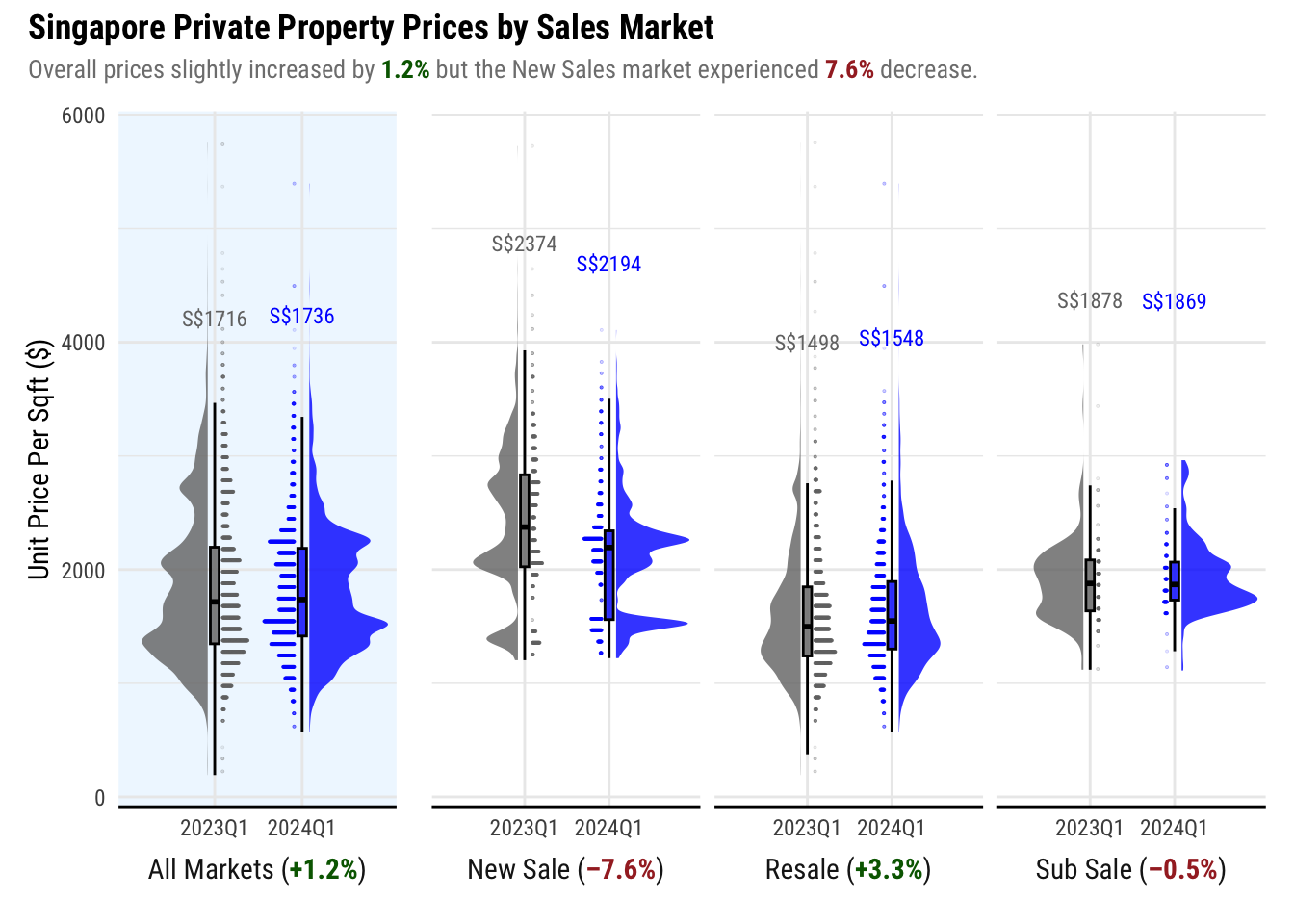
sales_txns_q1_24 <- sales_txns_q1_2324 %>% filter(QUARTER == "2024Q1")

4.2 Visualization 1: 2023Q1 and 2024Q1 prices

First we will compare the prices between the First Quarter of 2023 and 2024. This is to compare the prices at the same time of the year.

For this visualization, we will use the Unit Price per Sqft (UNIT_PRICE_PSF) instead of the Transaction Price (TRANSACTED_PRICE). This is so we can more fairly compare prices with less variables involved. With Transaction Price, the size of the property needs to be considered.

We will use the TYPE_OF_SALE column to partition the data so we can compare the trends across the Resale, New Sale and Sub Sale markets.

4.2.1 Creating the base Visualization

For the visualization, we will use a Raincloud Plot so that we can see the patterns in the price trends, and whether there are clusters of interest within the data set.

We will also add a boxplot to accompany the half-density plot so that we can see the quantiles more clearly.

To compare the different quarters, we will use both left side and right side visualization to compare the quarters side by side. This is inspired by a senior’s work.

To visualize the volumes, the 2 options are using stat_dots() or geom_jitter().

Raincloud Plot w/ volume plot (chosen)
Raincloud Plot w/ jitter plot (alternative)

Show ggplot2 code

plot_q1_yoy_psf_price <- function() {
  ggplot(
    sales_txns_q1_2324,
    aes(
      x = QUARTER,
      y = UNIT_PRICE_PSF,
      fill = QUARTER,
      color = QUARTER
    )
  ) +
    
    # Generate half-density plot
    stat_halfeye(
      aes(
        justification = ifelse(QUARTER == "2023Q1", 1.20, 0.02),
        side = ifelse(QUARTER == "2023Q1", "left", "right")
      ),
      position = position_nudge(x = 0.1, y = 0),
      .width = 0,
      alpha = 0.8,
      point_color = NA,
      show.legend = FALSE
    ) +
    
    # Generate boxplot along edge of half-density plot
    geom_boxplot(
      outlier.shape = NA,
      alpha = 0.8,
      width = .1,
      color = "black",
      show.legend = FALSE
    ) +
    
    # Generate volume plots, adjusting sizing so as to not overflow into the other half
    stat_dots(
      aes(
        side = ifelse(QUARTER == "2024Q1", "left", "right"),
        justification = ifelse(QUARTER == "2024Q1", 1.10,-0.1)
      ),
      binwidth = 100,
      dotsize = 0.005,
      alpha = 0.2,
      show.legend = FALSE
    ) +
    
    # Add text about the median price
    stat_summary(
      aes(label = paste0("S$", after_stat(y))),
      geom = "text",
      fun = "median",
      position = position_nudge(y = 2500),
      family = "Roboto Condensed",
      size = 3,
      show.legend = FALSE
    ) +
    
    # Set colors and fill
    # Keep it simple, and use bright color for 20424Q1 it is the focus of visualization
    scale_color_manual(values = c("grey45", "blue")) +
    scale_fill_manual(values = c("grey45", "blue")) +
    labs(y = "Unit Price Per Sqft ($)") +
    # Next steps will take care of theme enhancements
    theme_minimal()
}

plot_q1_yoy_psf_price()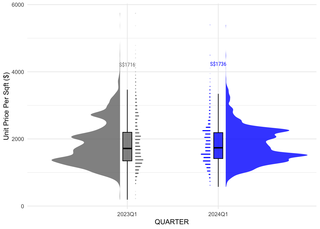

Show ggplot2 code

plot_q1_yoy_psf_price_alt <- function() {
  ggplot(
    sales_txns_q1_2324,
    aes(
      x = QUARTER,
      y = UNIT_PRICE_PSF,
      fill = QUARTER,
      color = QUARTER
    )
  ) +
    
    # Generate half-density plot
    stat_halfeye(
      aes(
        fill = QUARTER,
        justification = ifelse(QUARTER == "2023Q1", 1.22, 0),
        side = ifelse(QUARTER == "2023Q1", "left", "right")
      ),
      position = position_nudge(x = 0.1, y = 0),
      .width = 0,
      alpha = 0.8,
      point_color = NA,
      show.legend = FALSE
    ) +
    
    # Generate jitter plot under the geom plot so the dots don't overpower the boxplot
    geom_jitter(
      width = 0.08,
      size = 0.01,
      alpha = 0.2,
      show.legend = FALSE
    ) +
    
    # Generate boxplot along edge of half-density plot
    geom_boxplot(
      outlier.shape = NA,
      alpha = 0,
      width = 0.1,
      color = "black",
      show.legend = FALSE
    ) +
    
    # Add text about the median price
    stat_summary(
      aes(label = paste0("S$", after_stat(y))),
      geom = "text",
      fun = "median",
      position = position_nudge(y = 2500),
      family = "Roboto Condensed",
      size = 3,
      show.legend = FALSE
    )+
    
    # Set colors and fill
    # Keep it simple, and use bright color for 20424Q1 it is the focus of visualization
    scale_fill_manual(values = c("grey50", "blue")) +
    scale_color_manual(values = c("grey50", "blue")) +
    labs(y = "Unit Price Per Sqft ($)") +
    # Next steps will take care of theme enhancements
    theme_minimal()
}

plot_q1_yoy_psf_price_alt()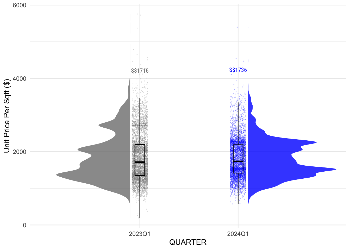

Decision: stat_dots()

Using stat_dots() is better than geom_jitter() as the purpose of providing volume information here is to accompany the half-density plot and provide a tool to compare the volume of each submarket.

Comparing the length of each horizontal line is much easier to do than comparing how dark each area is in a jitter plot.

Now that we have the base visualization, we will generate the final visualization.

4.2.2 Adding the % change

When generating the facet name, we also can add the % change so that it is clear for the audience how much the prices change.

We will use the following function to render the % change, which will show as +x.x% when there is an increase, and -x.x% when there is a decrease.

show_price_pc_change <- function(market = "1") {
  data2023 = sales_txns_q1_23
  data2024 = sales_txns_q1_24
  
  # 1 is the facet name for All markets
  if (market != "1") {
    data2023 = data2023 %>% filter(TYPE_OF_SALE == market)
    data2024 = data2024 %>% filter(TYPE_OF_SALE == market)
  } else {
    market = "All Markets"
  }
  
  median2023 = data2023$UNIT_PRICE_PSF %>% median()
  median2024 = data2024$UNIT_PRICE_PSF %>% median()
  
  sprintf(
    "%s (<span style='color:%s;'>**%s%0.1f%%**</span>)",
    market,
    ifelse(median2024 < median2023, "brown", "darkgreen"),
    ifelse(median2024 < median2023, "-", "+"),
    (median2024 - median2023) * 100 / median2023
  )
}

4.2.3 Generating the visualization

We want to compare the 2023 and 2024 Q1 sales for different submarkets. To do this, we will use facet_wrap() on TYPE_OF_SALE.

In addition, we will add another facet for All Markets for the overall comparison.

These 2 plots will be shown side by side using patchwork.

facet_grid(margin = TRUE) as alternative

We can also use facet_grid(margin = TRUE) to generate a facet with all the data, instead of generating 2 separate plots.

However, I would like to change the panel color for the overall plot to highlight it but I couldn’t find a way to do it within facet_grid().

Show ggplot2 code

q1_yoy_psf_price_submarkets_graph <- plot_q1_yoy_psf_price() +
  facet_wrap( ~ TYPE_OF_SALE,
              strip.position = "bottom",
              labeller = labeller(
                TYPE_OF_SALE = c(
                  "New Sale" = show_price_pc_change("New Sale"),
                  "Sub Sale" = show_price_pc_change("Sub Sale"),
                  "Resale" = show_price_pc_change("Resale")
                )
              )) +
  theme_minimal() +
  theme(axis.title.y = element_blank(),
        axis.text.y = element_blank())

q1_yoy_psf_price_all_markets_graph <- plot_q1_yoy_psf_price() +
  facet_wrap(
    ~ NUMBER_OF_UNITS,
    strip.position = "bottom",
    labeller = as_labeller(show_price_pc_change)
  ) +
  labs(x = "Transaction Price (,000 SGD)") +
  theme(panel.background = element_rect(fill = "aliceblue", linewidth =
                                          0))

# As much as we want the plot annotations to be dynamic, the subtitle is depending on the actual data
# Only this part is hardcoded
viz1 <- (q1_yoy_psf_price_all_markets_graph |
           q1_yoy_psf_price_submarkets_graph) +
  plot_layout(widths = c(1, 3)) +
  plot_annotation(title = "Singapore Private Property Prices by Sales Market",
                  subtitle = "Overall prices slightly increased by <span style='color:darkgreen;'>**1.2%**</span> but the New Sales market experienced <span style='color:brown;'>**7.6%**</span> decrease.") &
  theme(
    text = element_text(family = "Roboto Condensed"),
    axis.line.x = element_line(),
    axis.title.x = element_blank(),
    axis.ticks.y = element_blank(),
    plot.title = element_text(face = "bold"),
    plot.subtitle = element_markdown(color = "grey50", size = rel(0.9)),
    strip.placement = "outside",
    strip.text = element_markdown(size = rel(1))
  )
viz1

Insights

While the market generally saw a slight increase in unit prices from Q1 2023, the New Sale market experienced a decline. Notable clusters in the graph suggest concentrated sales around specific price points, likely influenced by factors such as developer pricing and the location of New Launches. According to data from 99.co, there are fewer than 10 New Launches in 2024.

New Launched projects, particularly big ones, resulted in clusters on certain price points as they introduce fresh supply in the districts they are located in. The demand for these properties also contributed to the trend as transactions are completed by buyers.

In contrast, the Resale Market, which is comprised of properties already turned over by developers, shows a smoother distribution of prices. This is attributed to the wider variation in prices negotiated between buyers and sellers on available properties all over Singapore, which is not constrained by the parameters of specific projects.

However, it is important to note that visualization can be very misleading especially on the New Sale Market. Generalizing that the trends when there are notable cluster may not be representative of the real state of the market.

Hence, we need to look more deeply into these groups and present it as a visualizations so it can be better understood why there are groups that formed.

4.3 Visualization 2: 2023Q1 and 2024Q1 Sales Volume

4.3.1 Understanding the groups in New Sales Market

We hypothesized that the groups that are present in the New Sales plot is due to the sales of newly-launched projects.

We will check the aggregated data by PROJECT_NAME and POSTAL_DISTRICT to verify our hypothesis that the sales are clustered by newly launched projects and their respective districts

By Project Name
By District

We will aggregate the number of sales and median unit price by projects. We will also add POSTAL_DISTRICT to the aggregation group as property prices depend on which district a property is in.

sales_txns_q1_24 %>% filter(TYPE_OF_SALE == "New Sale") %>% 
  group_by(POSTAL_DISTRICT, PROJECT_NAME) %>%
  summarize(
    MEDIAN_PRICE_PSF = median(UNIT_PRICE_PSF),
    NUMBER_OF_SALES = n()
  ) %>%
  arrange(desc(NUMBER_OF_SALES)) %>%
  head(10) %>% kable(row.name = TRUE)

	POSTAL_DISTRICT	PROJECT_NAME	MEDIAN_PRICE_PSF	NUMBER_OF_SALES
1	26	LENTOR MANSION	2269.0	409
2	23	LUMINA GRAND	1525.0	370
3	23	HILLHAVEN	2067.0	79
4	26	LENTORIA	2129.0	60
5	23	THE BOTANY AT DAIRY FARM	2019.0	59
6	27	NORTH GAIA	1326.5	54
7	12	THE ARCADY AT BOON KENG	2573.5	50
8	26	LENTOR HILLS RESIDENCES	2109.0	49
9	26	HILLOCK GREEN	2169.0	43
10	23	THE MYST	2160.5	42

We can see that 8 out of 10 projects with highest number of sales are in Districts 23 and 26. This is consistent with our previous observation that there are 2 groups in the New Sales density graph.

Furthermore, in 99.co’s New Launches page, Lentor Mansion (D26) and Lumina Grand (D23) are the biggest projects with the highest number of units sold.

Hence, the density graph could reflected the groups that formed from the sales of properties within these 2 projects.

sales_txns_q1_24 %>% filter(TYPE_OF_SALE == "New Sale") %>% 
  group_by(POSTAL_DISTRICT) %>%
  summarize(
    MEDIAN_PRICE_PSF = median(UNIT_PRICE_PSF),
    NUMBER_OF_SALES = n()
  ) %>%
  arrange(desc(NUMBER_OF_SALES)) %>%
  kable(row.names = TRUE)

	POSTAL_DISTRICT	MEDIAN_PRICE_PSF	NUMBER_OF_SALES
1	23	1542.0	576
2	26	2253.0	571
3	15	2615.5	72
4	21	2453.0	57
5	27	1328.0	56
6	12	2573.0	51
7	11	3189.0	40
8	10	3307.0	37
9	03	2807.0	31
10	05	2607.5	20
11	28	2254.0	20
12	16	2091.0	19
13	22	2215.0	17
14	09	3437.5	14
15	02	2567.0	13
16	07	3234.0	8
17	19	1966.0	7
18	14	2168.0	5
19	18	1754.0	3
20	04	2548.5	2
21	17	1895.0	2

Although there are new units across all districts, the big, newly launched projects contributed the most to the New Sales Market.

This is hinted by the fact that after aggregating all property sales by district, D23 and D26 where Lumina Grand and Lentor Mansion stand out. More than 60% of sales from each of these district also come from these 2 projects.

Based on the findings from this deep dive, we will visualize the sales volume by district.

4.3.2. Creating the base visualization

Some of the options we have to visualize the sales by district are:

Bar graph of number of sales for all districts, or
Bar graph of number of sales for most popular districts

All districts
Most popular districts (chosen)

plot_q1_yoy_sale_vol <- function() {
ggplot(
  sales_txns_q1_2324,
  aes(x = POSTAL_DISTRICT, fill = QUARTER)
) +
  geom_bar(position="dodge", show.legend = FALSE) +
  coord_flip() +
  scale_fill_manual(values = c("grey45", "blue")) +
  theme_minimal()
}

plot_q1_yoy_sale_vol()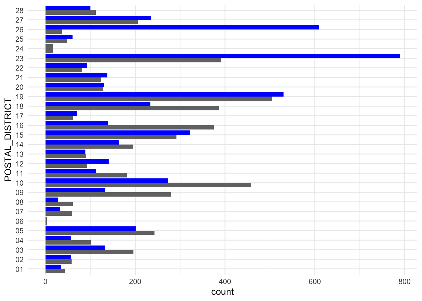

This visualization needs some pre-processing so we can determine the Top 5 most popular districts in each submarket.

popular_districts <- sales_txns_q1_2324 %>% 
  group_by(QUARTER, POSTAL_DISTRICT, TYPE_OF_SALE) %>%
  summarize(
    MEDIAN_PRICE_PSF = median(UNIT_PRICE_PSF),
    NUMBER_OF_SALES = n()
  ) %>%
  group_by(QUARTER, TYPE_OF_SALE) %>%
  arrange(desc(NUMBER_OF_SALES)) %>%
  mutate(RANK = order(NUMBER_OF_SALES, decreasing=TRUE)) %>%
  filter(RANK <= 5) %>%
  select(c(QUARTER, TYPE_OF_SALE, RANK, POSTAL_DISTRICT, NUMBER_OF_SALES, MEDIAN_PRICE_PSF)) %>%
  arrange(QUARTER)

kable(popular_districts, row.names = TRUE)

	QUARTER	TYPE_OF_SALE	RANK	POSTAL_DISTRICT	NUMBER_OF_SALES	MEDIAN_PRICE_PSF
1	2023Q1	Resale	1	19	401	1337.0
2	2023Q1	Resale	2	15	260	1830.0
3	2023Q1	Resale	3	10	251	2162.0
4	2023Q1	Resale	4	16	210	1410.5
5	2023Q1	Resale	5	23	208	1258.5
6	2023Q1	New Sale	1	10	202	2942.5
7	2023Q1	New Sale	2	23	178	2071.5
8	2023Q1	New Sale	3	18	168	1390.0
9	2023Q1	New Sale	4	16	165	2084.0
10	2023Q1	New Sale	5	09	150	2846.0
11	2023Q1	Sub Sale	1	19	54	1635.5
12	2023Q1	Sub Sale	2	14	34	2096.5
13	2023Q1	Sub Sale	3	13	27	1913.0
14	2023Q1	Sub Sale	4	18	24	1598.0
15	2023Q1	Sub Sale	5	05	19	1912.0
16	2024Q1	New Sale	1	23	576	1542.0
17	2024Q1	New Sale	2	26	571	2253.0
18	2024Q1	Resale	1	19	429	1448.0
19	2024Q1	Resale	2	15	243	1719.0
20	2024Q1	Resale	3	10	236	2171.5
21	2024Q1	Resale	4	23	209	1361.0
22	2024Q1	Resale	5	18	182	1350.0
23	2024Q1	Sub Sale	1	19	94	1771.5
24	2024Q1	New Sale	3	15	72	2615.5
25	2024Q1	New Sale	4	21	57	2453.0
26	2024Q1	New Sale	5	27	56	1328.0
27	2024Q1	Sub Sale	2	05	53	2061.0
28	2024Q1	Sub Sale	3	18	49	1694.0
29	2024Q1	Sub Sale	4	13	20	2044.0
30	2024Q1	Sub Sale	5	14	14	2051.5

Now that we have this aggregated dataset, we can use this to plot the ranked data. For example, we can plot the most popular districts in the New Sales Market.

ggplot(popular_districts %>% filter(TYPE_OF_SALE =="New Sale"),
       aes(x = reorder(RANK, -RANK), y = NUMBER_OF_SALES, fill = QUARTER))+
  geom_bar(stat="identity", position = "dodge", show.legend = FALSE, alpha =0.8) +
  geom_text(aes(y = 10, hjust=0, label=paste0("D", POSTAL_DISTRICT, ": ", NUMBER_OF_SALES))) +
  coord_flip(ylim= c(0, 600)) +
  scale_fill_manual(values = c("grey45", "blue")) +
  facet_wrap(~QUARTER)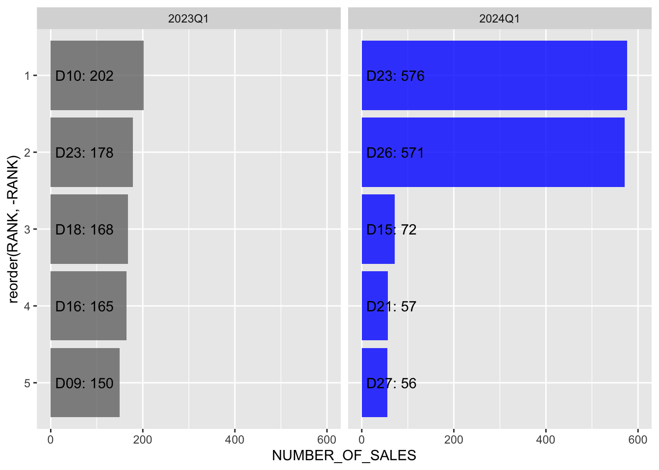

With this visualization, we can compare the top districts from 2 quarters side by side.

From the 2 options, plotting the Most Popular Districts is more appropriate for our use case. This is because we would like the user to recognize which districts are driving the price trends.

When we plot all the districts, it is more difficult to identify by sight which districts are popular in a quarter and the other. This is because this plot has a lot of noise, which may not be that relevant to connect to the previous visualization.

4.3.3 Generating the visualization

We will generate the visualization such that QUARTER is in column and TYPE_OF_SALE is in rows.

We will using facet_grid() to generate the visualization and adjust the theme elements as needed to make the plot more presentable.

Show ggplot2 code

viz2 <- ggplot(popular_districts,
       aes(
         # Order the axis elements by rank
         x = reorder(RANK,-RANK),
         y = NUMBER_OF_SALES,
         fill = QUARTER
       )) +
  
  # Generate bar graph based on number of sales
  geom_bar(
    stat = "identity",
    position = "dodge",
    show.legend = FALSE,
    alpha = 0.8
  ) +
  
  # Add descriptive label
  geom_text(aes(
    y = 10,
    hjust = 0,
    label = sprintf(
      "D%s: %d units sold at S$%0.2f psf",
      POSTAL_DISTRICT,
      NUMBER_OF_SALES,
      MEDIAN_PRICE_PSF
    )
  ), family = "Roboto Condensed") +
  
  # Generate horizontal bar
  coord_flip(ylim = c(0, 600)) +
  
  # Set colors consistent with previous visualization
  scale_fill_manual(values = c("grey45", "blue")) +
  
  # Generate facets, with labels to the left and at the bottom
  facet_grid(TYPE_OF_SALE ~ QUARTER, switch = "both") +
  
  # Set plot texts
  plot_annotation(title = "Districts With Highest Units Sold for Each Submarket",
                  subtitle = "New Sale Market is heavily influenced by the newly-launched projects in **D23** (Lumina Grand) and **D26** (Lentor Mansion).",
                  caption = "Prices shown are **median unit price** per sqft") &
  # Set theme
  theme_minimal() +
  theme(
    text = element_text(family = "Roboto Condensed"),
    axis.line.x = element_line(),
    axis.title.x = element_blank(),
    axis.title.y = element_blank(),
    axis.text.y = element_blank(),
    plot.title = element_text(face = "bold"),
    # Use element_markdown so we can style the text
    plot.subtitle = element_markdown(color = "grey50", size = rel(0.9)),
    plot.caption = element_markdown(color = "grey50"),
    strip.placement = "outside",
    strip.text = element_text(size = rel(1))
  )
viz2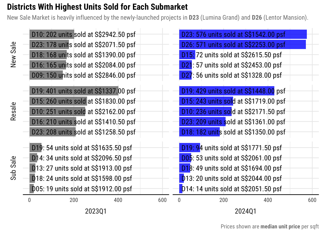

About the texts in the visualization

Texts such as xx units sold at $xxxx.xx were added in the plot so the information is easily digestible.

However, it made the plot messy, and not aesthetically pleasing. Ideally, the full text should be rendered when interacting with the graph. I do not know how to do that right now, but it will be how I will present this visualization in the future.

Given this limit in my present abilities, I prioritized clarity of information over aesthetic considerations.

Insights

Plotting the most popular districts for each submarket reveals that the Top 5 districts in the New Sale market, differs for the 2 quarters.

In 2023Q1, the distribution is more balanced and there were a lot of units sold in expensive districts like Districts 9 and 10. However, In 2024Q1, the number of units sold were skewed towards cheaper districts like Districts 23 and 26 where big projects like Lumina Grand and Lentor Mansion, respectively, were launched.

This is why the overall prices in the New Sale market appear to be much cheaper than the previous year, when in fact the new projects that launched are in cheaper districts.

On the contrary, the top districts in the Resale and Sub Sale markets have much less difference. This smaller change also resulted in a smaller impact on the overall median price in these markets.

4.4 Visualization 3: 2024 Q1 Market by Property Type

4.4.1 Checking price trends by property type

Previous visualizations focused on comparisons between the Q1 of 2023 and 2024, and based on the different markets.

For the next visualization, we will first explore the data with 2024Q1, based on the property type.

Let us group the data by TYPE_OF_SALE and PROPERTY_TYPE if we can gain new insights based on the size of property. We will get the aggregated median values for price and area columns.

sales_txns_q1_24 %>%
  group_by(TYPE_OF_SALE, PROPERTY_TYPE) %>%
  summarize(
    UNIT_PRICE_PSF = median(UNIT_PRICE_PSF),
    TRANSACTED_PRICE = median(TRANSACTED_PRICE),
    AREA_SQFT = median(AREA_SQFT),
    UNITS_SOLD = n()
  ) %>% arrange(desc(UNITS_SOLD), .by_group = TRUE) %>%
  kable

TYPE_OF_SALE	PROPERTY_TYPE	UNIT_PRICE_PSF	TRANSACTED_PRICE	AREA_SQFT	UNITS_SOLD
New Sale	Apartment	2277.0	1908500	796.540	864
New Sale	Executive Condominium	1516.0	1515000	995.670	448
New Sale	Condominium	2204.0	2083000	990.290	290
New Sale	Terrace House	2254.0	3655000	1614.600	17
New Sale	Detached House	1790.0	11690000	6607.855	2
Resale	Condominium	1580.5	1660000	1119.460	1480
Resale	Apartment	1718.5	1460000	893.410	796
Resale	Executive Condominium	1305.0	1375000	1076.400	395
Resale	Terrace House	1751.0	3750000	2055.920	197
Resale	Semi-Detached House	1665.0	5642500	3459.010	92
Resale	Detached House	1503.0	10940000	7004.130	38
Sub Sale	Apartment	1914.0	1473000	721.190	193
Sub Sale	Condominium	1772.5	1525000	742.720	88
Sub Sale	Terrace House	1482.5	3229000	2195.855	2
Sub Sale	Semi-Detached House	1171.0	4750000	4058.030	1

From this aggregated data, we can see that Executive Condominiums are relatively cheaper than Condominiums and Apartments, which are of similar area. From my research, Executive Condominiums are under HDB, but are built and sold by property developers. This is why it is much cheaper.

We can also notice that there are much lower sales for some property types, like Terrace House, Semi-Detached House, and Detached House. These are landed properties, which are quite rare in Singapore so it is logical to see much fewer sales of these properties.

4.4.2 Creating base visualizations

From the insights gained from our initial exploration, we observed that prices differ by property types and that there are less sales on some property prices.

Unit Price
Volume

For the unit price, we will use boxplot instead of density plots as we can see the distribution for different markets. If we use density plots, it is harder to present partitioned data in an easy to understand way.

Lastly, we will generate some reference lines for statistics (mean and median).

Show ggplot2 code

# Calculate stats for reference lines
median_q1 <- median(sales_txns_q1_24$UNIT_PRICE_PSF)
mean_q1 <- mean(sales_txns_q1_24$UNIT_PRICE_PSF)

unit_price_by_prop_type <- ggplot(sales_txns_q1_24,
                                  aes(x = PROPERTY_TYPE, y = UNIT_PRICE_PSF, fill = TYPE_OF_SALE)) +
  
  # Generate different boxplots for each market and property type
  geom_boxplot(outliers = FALSE,
               width = 0.4,
               alpha = 0.8) +
  
  # Render median reference line
  geom_hline(aes(yintercept = median_q1, color = "Median"),
             linetype = "dashed",
             alpha = 0.8) +
  annotate(
    geom = "text",
    x = 6.6,
    y = ifelse(median_q1 < mean_q1, median_q1 - 200, median_q1 + 250),
    label = paste0("Median =\n$", median_q1),
    family = "Roboto Condensed",
    color = "brown",
    size = 3,
    alpha = 0.8
  ) +
  
  # Render mean reference line
  geom_hline(aes(yintercept = mean_q1, color = "Mean"),
             linetype = "dashed",
             alpha = 0.8) +
  annotate(
    geom = "text",
    x = 6.6,
    y = ifelse(mean_q1 < median_q1, mean_q1 - 200, mean_q1 + 250),
    label = paste0("Mean =\n$", round(mean_q1, 0)),
    family = "Roboto Condensed",
    color = "darkgreen",
    size = 3,
    alpha = 0.8
  ) +
  
  # Set labels
  labs(x = "Property Type",
       y = "Unit Price Per Sqft ($)",
       fill = "Market",
       color = "Statistics") +
  
  # Wrap long labels using `wrap_format()` from `scale` package
  # Add some space to the right for Statistics annotations
  scale_x_discrete(labels = wrap_format(10), expand = expansion(add = c(0.6, 1))) +
  
  # Set colors
  scale_fill_manual(values = c("darkorange", "blue", "gold3")) +
  scale_color_manual(values = c("darkgreen", "brown")) +
  theme_minimal() +
  theme(
    # Remove axis text. Combining this with the price visualization will stack the 2 graphs
    axis.text.x = element_blank()
  )

unit_price_by_prop_type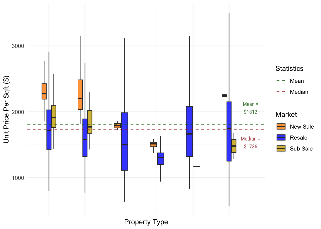

We can see from the graph that some box plots are very short, which is especially true for Landed properties as there are few units sold for these property types.

As companion to the unit price graph, we will also generate a simple bar graph for the volume.

Show ggplot2 code

sales_volume_by_prop_type <-
  ggplot(
    sales_txns_q1_24,
    aes(x = PROPERTY_TYPE, fill = TYPE_OF_SALE)
  ) +
  
  # Generate stacked bar graph by TYPE_OF_SALE
  # Do not show label as the price graph will show it
  geom_bar(alpha = 0.8, width = 0.5, show.legend = FALSE) +
  
  # Generate labels for stacked bar areas
  # Do not show label as the price graph will show it
  # Use ggrepel as some areas in the bar graph are too small to render th text inside
  geom_label_repel(
    aes(label = after_stat(count)),
    stat = "count",
    position = "stack",
    family = "Roboto Condensed",
    size = 2.5,
    alpha = 0.8,
    color = "white",
    show.legend = FALSE
  ) +
  
  # Apply colors
  scale_fill_manual(values = c("darkorange", "blue", "gold3")) +
  labs(y = "Units Sold") +
  
  # Wrap long titles
  # Apply same "expand" so axes align
  scale_x_discrete(labels = wrap_format(10), expand = expansion(add = c(0.6, 1))) +
  
  # Appply theme
  theme_minimal() +
  theme()

sales_volume_by_prop_type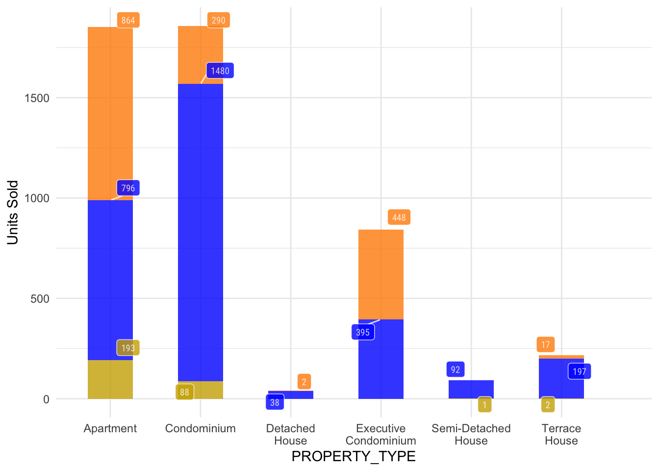

The volume graph provides additional information about sales by property type. Some property types with lower sales volume may show a longer boxplot, which may be interpreted as more units sold.

With this companion graph, it is easier to cross-reference the price with the volume to better judge how representative of the market the unit prices are.

4.4.3 Generating the visualization

Finally, we will generate the visualization by stacking the 2 graphs and doing final touches on the styling and texts.

Show ggplot2 code

viz3 <- (unit_price_by_prop_type / sales_volume_by_prop_type ) +
  plot_layout(heights = c(5,1)) +
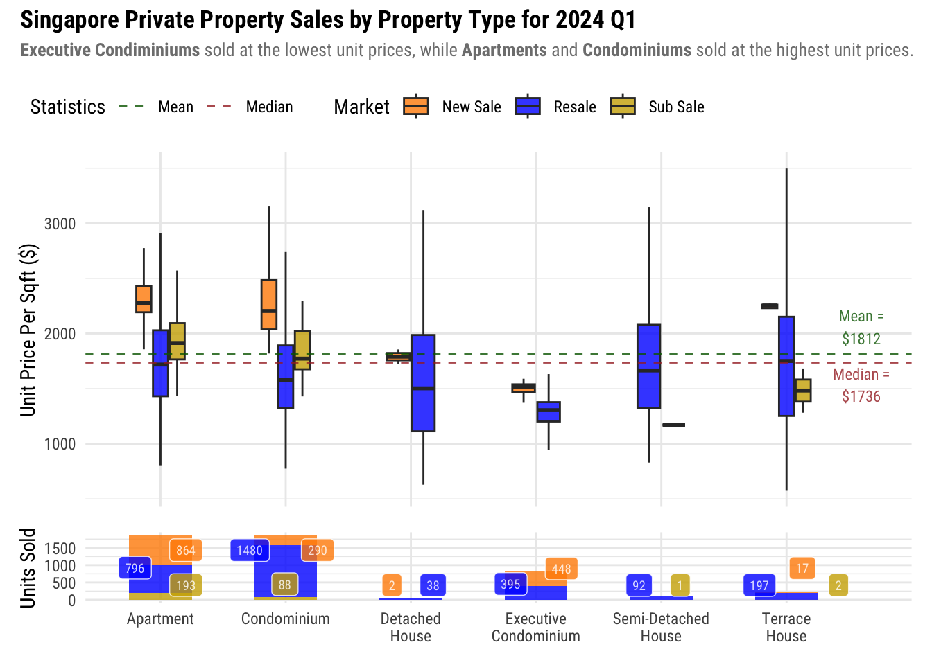
  plot_annotation(title = "Singapore Private Property Sales by Property Type for 2024 Q1",
                  subtitle = "**Executive Condiminiums** sold at the lowest unit prices, while **Apartments** and **Condominiums** sold at the highest unit prices.") &
  theme(
    text = element_text(family = "Roboto Condensed"),
    axis.title.x = element_blank(),
    legend.position = "top",
    legend.justification = "left",
    legend.location = "plot",
    plot.title = element_text(face = "bold"),
    plot.subtitle = element_markdown(color = "grey50", size = rel(0.9)),
  )
viz3

Insights

From our initial exploration, we have already established that Executive Condominiums are cheapest in terms of unit price.

Another surprising observation is that despite having more Executive Condominiums sold, its boxplot is notably shorter compared to Detached and Semi-Detached Houses, in both the New Sale and Resale Markets. This disparity may be attributed to HDB’s price regulation on Executive Condominiums, resulting in reduced price variability compared to other property types.

It can also be observed that there are much fewer sales in the New Sales market of landed properties. It could be due to the fact that compared to Strata developments, Landed properties are usually bespoke to their owner’s use. In addition to the fact that landed properties are rare in Singapore, is it expected to see less New Sales in this category.

Lastly, the mean is higher than the median price which means that the unit prices are skewed towards the higher end of the scale. What this means it that prices tend to be more expensive than cheaper.

5 Summary

5.1 Visualizations

For this exercise, we generated 3 visualizations, show below.

5.1.1 Singapore Private Property Prices by Sales Market

5.1.2 Districts with Highest Units Sold for Each Submarket

5.1.3 Singapore Private Property Sales by Property Type for 2024 Q1

5.2 Overall Insights

We found that the 2024 New Sales market experienced an sizable decrease is overall prices (7.6%) compared to the same period last year. However, it should be noted that this is due to New Launches located in cheaper districts, compared to the same period last year where that launches where in central districts like 9 and 10.

Another very interesting insight is that different property prices experience big variations in prices, while Executive Condominiums have smaller variations. This is because of the more controlled and regulated environment as these properties are under the jurisdiction of HDB. This is why although median prices are at S$1736 in 2024Q1, it is possible to find a more affordable property when looking at Executive Condominiums.

Hence, a prospective buyer must take generalizations in the housing market with the grain of salt as overall market trends may not reflect the situation in the market they are interested in. This is why when thinking of buying a property, it is important to be more specific on the kind of property you are looking for (e.g. which district, property type, new or resale, etc) and narrow down on the trends for each of those. They must do their own due diligence in researching the market they are interested in to make a sound decision on their purchase.

5.3 Reflections

When choosing how to visualize the data, I had to make hard decisions on what data subsets to select. At first I was wary that I will be presenting misleading data. My own bias and limitations also reflect the output as I had to limit myself to looking at 2 quarters as I cannot imagine how to present data from all 5 quarters effectively with the level of detail in the different submarkets and property type.

However, I realized that with the details available to us, it is impossible to cover everything. It is more important to tailor the visualization to our target audience, and even then we may not be able to provide everything they need.

I am now more aware that as a data visualization consumer, I must do my on due diligence to dive deep into the details as the visualizations may be too general or too detailed for our own needs. Some data may be omitted or data due to various limitations.

As a student, there were also some frustrating moments as I wanted to present data in a certain way but my current abilities limit me from presenting data in such a way (especially on Visualization 2). As I progress in this course, I will challenge myself to implement those ideas as I expand my own learning.

6 References

99.co. (2024). New Launch Condos & Projects in Singapore. 99.co. https://www.99.co/singapore/new-launches

Holtz, Yan. (2024). Dealing with colors in ggplot2. The R Graph Gallery. https://r-graph-gallery.com/ggplot2-color.html

Housing & Development Board. (2024). Executive Condominium. Housing & Development Board. https://www.hdb.gov.sg/residential/buying-a-flat/executive-condominium

Kam, Tin Seong. (2023). Visualising Distribution. R for Visual Analytics. https://r4va.netlify.app/chap09

Lim, Abram. (2024). 13+ Housing & Household Statistics in Singapore (2024).SmartWealth Singapore. https://smartwealth.sg/housing-household-statistics-singapore/

PropertyGuru Editorial Team. (2024). Singapore Property Market Outlook 2024 Overview. PropertyGuru. https://www.propertyguru.com.sg/property-guides/singapore-property-market-outlook-2024-90041

Tan, Kylie. (2023). Take-home Exercise 1: Investigating Student Performance with Data Visualisations. Kale’s Visual Analytics Tales. https://akalestale.netlify.app/

Trading Economics. (2024). Home Ownership Rate | G20. https://tradingeconomics.com/country-list/home-ownership-rate?continent=g20