pacman::p_load(tidytext, widyr, wordcloud, DT, ggwordcloud, textplot, lubridate, hms, tidyverse, tidygraph, ggraph, igraph)

# Set seed
set.seed(1234)Hands-on Exercise 5: Visualizing and Analyzing Text Data
1 Overview
This hands-on exercise covers Chapter 29: Visualising and Analysing Text Data with R: tidytext methods.
I learned about the following:
understand tidytext framework for processing, analysing and visualising text data,
write function for importing multiple files into R,
combine multiple files into a single data frame,
clean and wrangle text data by using tidyverse approach,
visualize words with Word Cloud,
compute term frequency–inverse document frequency (TF-IDF) using tidytext method, and
visualizing texts and terms relationship.
2 Getting Started
2.1 Loading the required packages
For this exercise we will use the following R packages:
tidytext, tidyverse (mainly readr, purrr, stringr, ggplot2)
widyr,
wordcloud and ggwordcloud,
textplot (required igraph, tidygraph and ggraph, )
DT,
lubridate and hms
2.2 Importing Multiple Text Files from Multiple Folders
2.2.1 Creating a folder list
news20 <- "data/20news"2.2.2 Define a function to read all files from a folder into a data frame
read_folder <- function(infolder) {
  tibble(file = dir(infolder,
                    full.names = TRUE)) %>%
    mutate(text = map(file,
                      read_lines)) %>%
    transmute(id = basename(file),
              text) %>%
    unnest(text)
}
2.3 Importing Multiple Text Files from Multiple Folders
2.3.1 Reading in all the messages from the 20news folder
raw_text <- tibble(folder =
                     dir(news20,
                         full.names = TRUE)) %>%
  mutate(folder_out = map(folder,
                          read_folder)) %>%
  unnest(cols = c(folder_out)) %>%
  transmute(newsgroup = basename(folder),
            id, text)
write_rds(raw_text, "data/rds/news20.rds")
3 Initial EDA
We can visualize the frequency of messages by newsgroup.
raw_text %>%
  group_by(newsgroup) %>%
  summarize(messages = n_distinct(id)) %>%
  ggplot(aes(messages, newsgroup)) +
  geom_col(fill = "lightblue") +
  labs(y = NULL)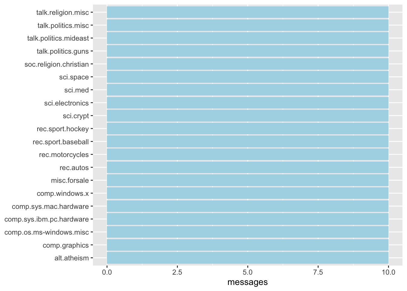
For each newsgroup, there are 10 different ids
4 Introducing tidytext
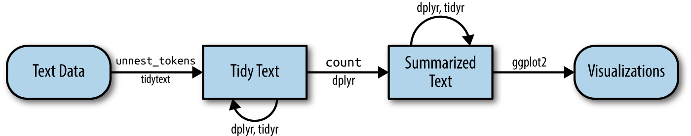
Using tidy data principles in processing, analysing and visualising text data.
Much of the infrastructure needed for text mining with tidy data frames already exists in packages like ‘dplyr’, ‘broom’, ‘tidyr’, and ‘ggplot2’.
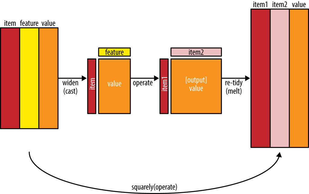
Figure below shows the workflow using tidytext approach for processing and visualising text data.
4.1 Removing header and automated email signitures
Each message has some structure and extra text that we don’t want to include in our analysis. For example, every message has a header, containing field such as “from:” or “in_reply_to:” that describe the message. Some also have automated email signatures, which occur after a line like “–”.
cleaned_text <- raw_text %>%
  group_by(newsgroup, id) %>%
  filter(cumsum(text == "") > 0,
         cumsum(str_detect(
           text, "^--")) == 0) %>%
  ungroup()
This code chunk removes the non-message texts from the raw texts.
4.2 Removing lines with nested text representing quotes from other users
cleaned_text <- cleaned_text %>%
  filter(str_detect(text, "^[^>]+[A-Za-z\\d]")
         | text == "",
         !str_detect(text,
                     "writes(:|\\.\\.\\.)$"),
         !str_detect(text,
                     "^In article <")
  )
This removed quotes from other users so they are not double counted/analyzed.
4.3 Text Data Processing
In this code chunk below, unnest_tokens() of tidytext package is used to split the dataset into tokens, while stop_words is used to remove stop-words.
usenet_words <- cleaned_text %>%
  unnest_tokens(word, text) %>%
  filter(str_detect(word, "[a-z']$"),
         !word %in% stop_words$word)
Now that we’ve removed the headers, signatures, and formatting, we can start exploring common words. For starters, we could find the most common words in the entire dataset, or within particular newsgroups.
usenet_words %>%
  count(word, sort = TRUE) %>% datatable()
Instead of counting individual word, we can also count words within by newsgroup by using the code chunk below.
words_by_newsgroup <- usenet_words %>%
  count(newsgroup, word, sort = TRUE) %>%
  ungroup()
words_by_newsgroup %>% datatable()
4.4 Visualising Words in newsgroups using wordcloud package
We can also add colors. For convenience, we can use palettes from brewer.
wordcloud(words_by_newsgroup$word,
          words_by_newsgroup$n,
          max.words = 300,
          colors = brewer.pal(9,"Dark2"))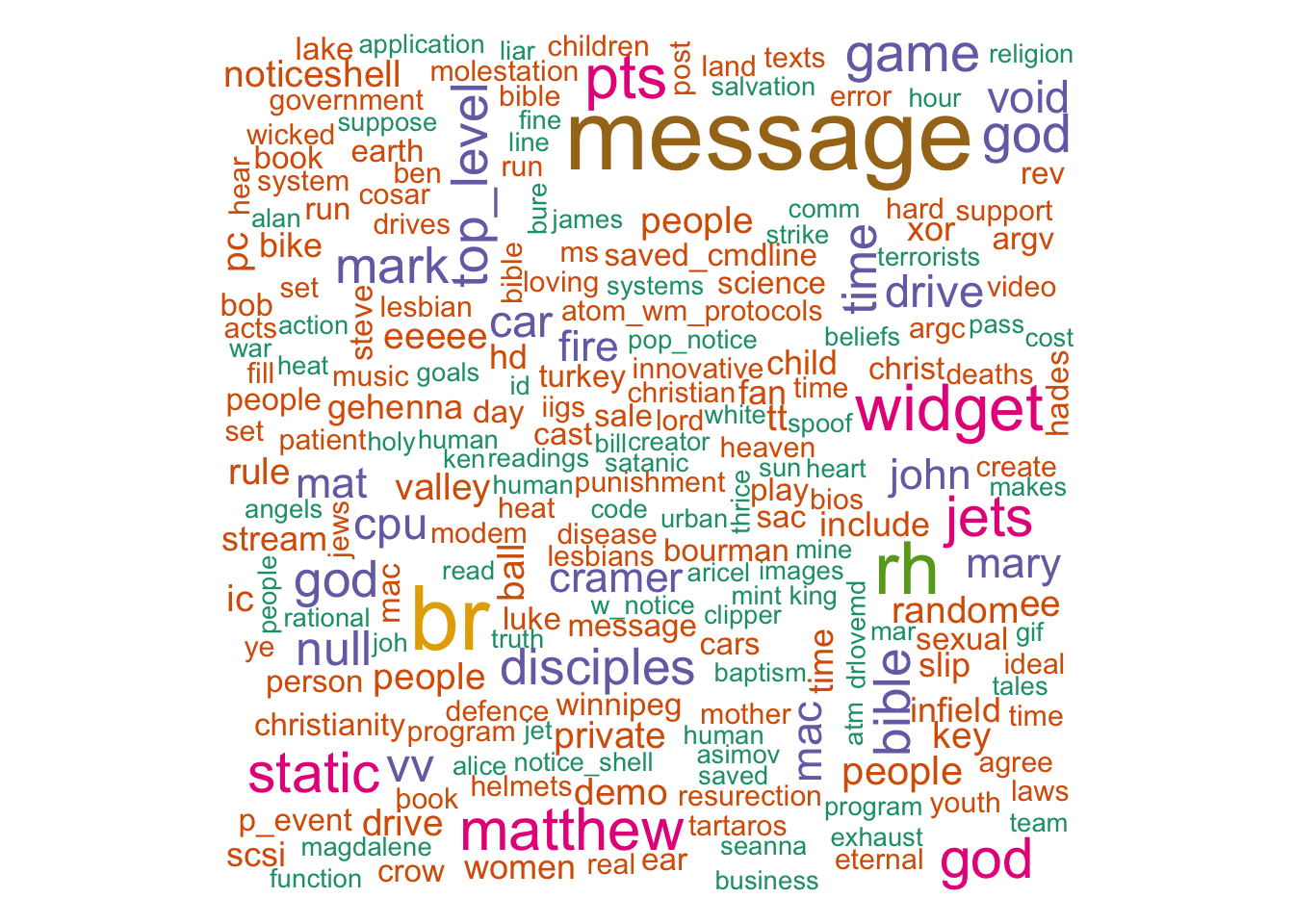
A DT table can be used to complement the visual discovery. We specify filter to add text filter per column.
datatable(words_by_newsgroup, filter = "top")4.5 Visualising Words in newsgroups using ggwordcloud package
This can be used along with ggplot2. In the code below, we render facets for each newsgroup to visualize the words per news group.
Note: Specified n > 8 so wordcloud renders faster and texts do not overlap.
words_by_newsgroup %>%
  filter(n > 8) %>%
ggplot(aes(label = word,
           size = n)) +
  geom_text_wordcloud() +
  theme_minimal() +
  facet_wrap(~newsgroup)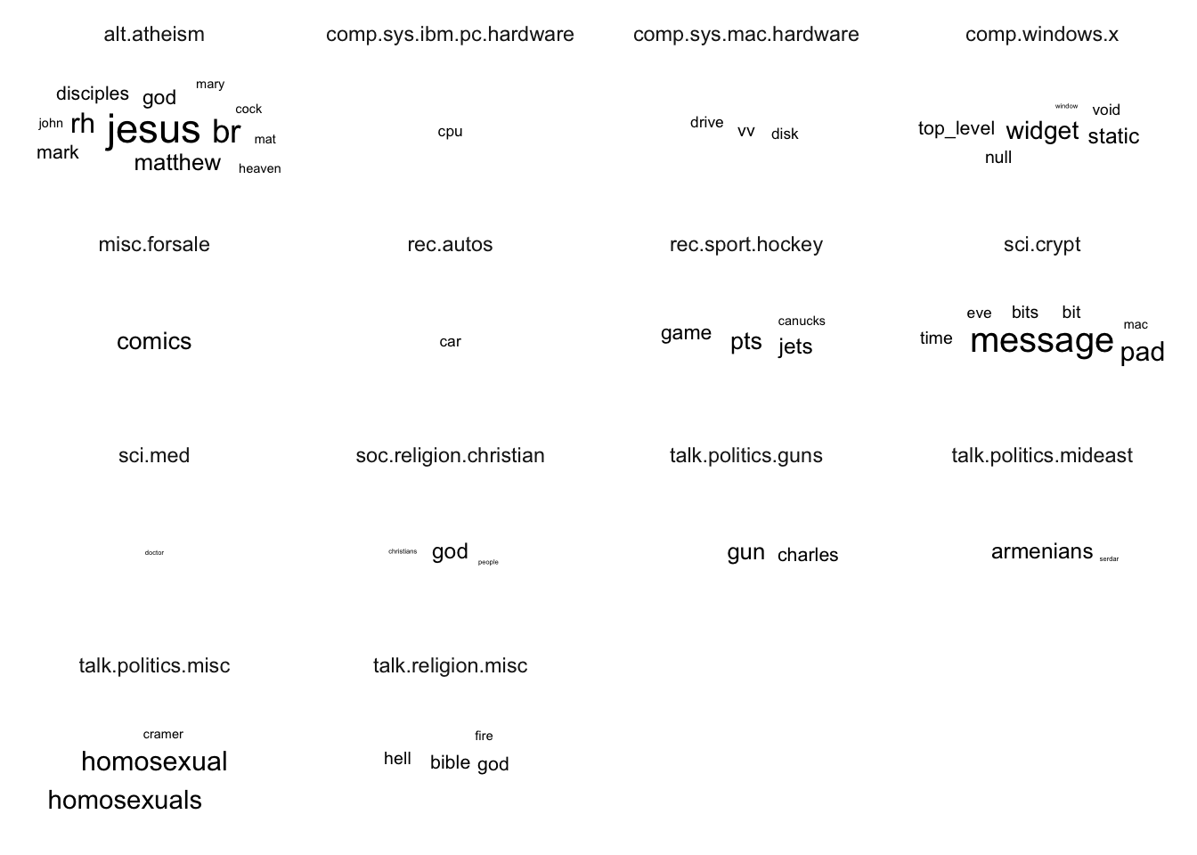
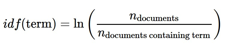
5 Basic Concept of TF-IDF
- tf–idf, short for term frequency–inverse document frequency, is a numerical statistic that is intended to reflect how important a word is to a document in a collection of corpus.
5.1 Computing tf-idf within newsgroups
The code chunk below uses bind_tf_idf() of tidytext to compute and bind the term frequency, inverse document frequency and ti-idf of a tidy text dataset to the dataset.
tf_idf <- words_by_newsgroup %>%
  bind_tf_idf(word, newsgroup, n) %>%
  arrange(desc(tf_idf))
5.2 Visualising tf-idf as interactive table
Table below is an interactive table created by using datatable().
We can also use formatRound() to format columns, according to the docs. We can also use formatStyle() to add some styling.
datatable(tf_idf, filter = "top") %>%
  formatRound(c("tf", "idf", "tf_idf"), 3) %>%
  formatStyle(0,
              target = 'row',
              lineHeight='25%')
5.3 Visualising tf-idf within newsgroups
Facet bar charts technique is used to visualise the tf-idf values of science related newsgroup.
tf_idf %>%
  filter(str_detect(newsgroup, "^sci\\.")) %>%
  group_by(newsgroup) %>%
  slice_max(tf_idf,
            n = 12) %>%
  ungroup() %>%
  mutate(word = reorder(word,
                        tf_idf)) %>%
  ggplot(aes(tf_idf,
             word,
             fill = newsgroup)) +
  geom_col(show.legend = FALSE) +
  facet_wrap(~ newsgroup,
             scales = "free") +
  labs(x = "tf-idf",
       y = NULL)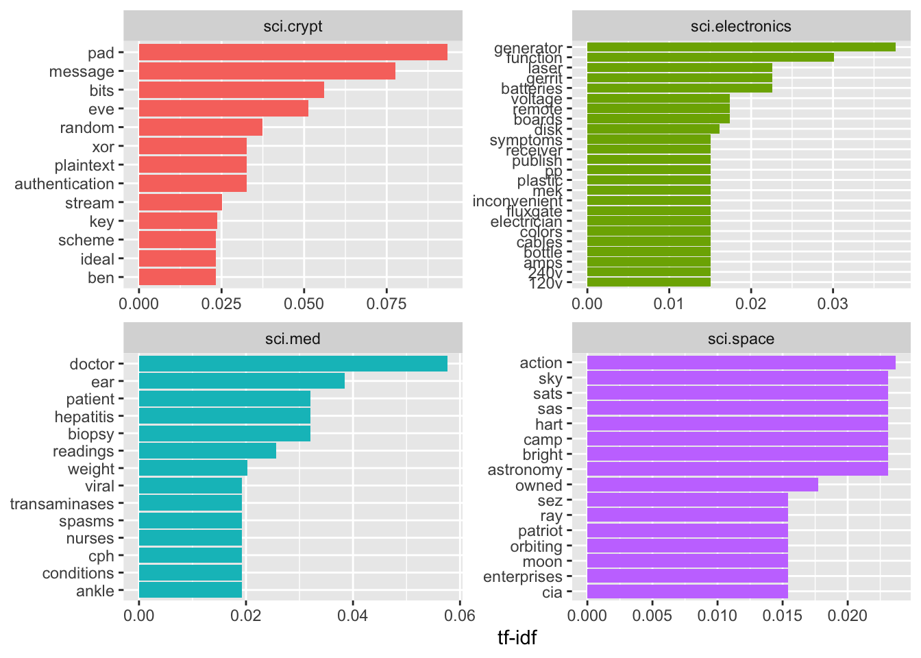
6 Word Correlations
6.1 Counting and correlating pairs of words with the widyr package
To count the number of times that two words appear within the same document, or to see how correlated they are.
Most operations for finding pairwise counts or correlations need to turn the data into a wide matrix first.
widyr package first ‘casts’ a tidy dataset into a wide matrix, performs an operation such as a correlation on it, then re-tidies the result.
In this code chunk below, pairwise_cor() of widyr package is used to compute the correlation between newsgroup based on the common words found.
newsgroup_cors <- words_by_newsgroup %>%
  pairwise_cor(newsgroup,
               word,
               n,
               sort = TRUE)
6.2 Visualising correlation as a network
Now, we can visualise the relationship between newgroups in network graph as shown below.
newsgroup_cors %>%
  filter(correlation > .025) %>%
  graph_from_data_frame() %>%
  ggraph(layout = "fr") +
  geom_edge_link(aes(alpha = correlation,
                     width = correlation)) +
  geom_node_point(size = 6,
                  color = "lightblue") +
  geom_node_text(aes(label = name),
                 color = "red",
                 repel = TRUE) +
  theme_void()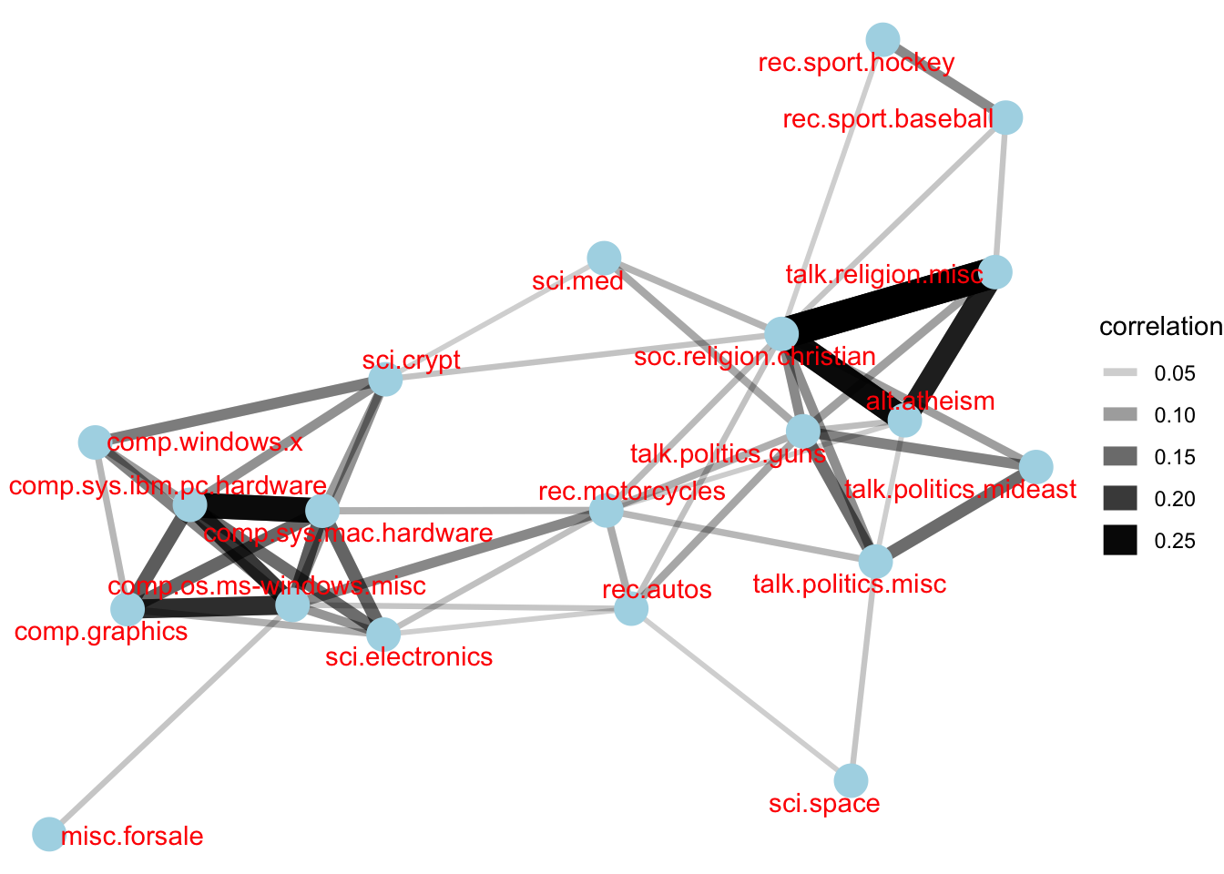
Result differs from the original chapter as we are using seed 1234 instead of 2017.
6.3 Bigram
In this code chunk below, a bigram data frame is created by using unnest_tokens() of tidytext.
bigrams <- cleaned_text %>%
  unnest_tokens(bigram,
                text,
                token = "ngrams",
                n = 2)
bigrams
# A tibble: 28,824 × 3
newsgroup id bigram
<chr> <chr> <chr>
1 alt.atheism 54256 <NA>
2 alt.atheism 54256 <NA>
3 alt.atheism 54256 as i
4 alt.atheism 54256 i don't
5 alt.atheism 54256 don't know
6 alt.atheism 54256 know this
7 alt.atheism 54256 this book
8 alt.atheism 54256 book i
9 alt.atheism 54256 i will
10 alt.atheism 54256 will use
# ℹ 28,814 more rows6.4 Counting bigrams
The code chunk is used to count and sort the bigram data frame ascendingly.
bigrams_count <- bigrams %>%
  filter(bigram != 'NA') %>%
  count(bigram, sort = TRUE)
bigrams_count
# A tibble: 19,885 × 2
bigram n
<chr> <int>
1 of the 169
2 in the 113
3 to the 74
4 to be 59
5 for the 52
6 i have 48
7 that the 47
8 if you 40
9 on the 39
10 it is 38
# ℹ 19,875 more rows6.5 Cleaning bigram
The code chunk below is used to seperate the bigram into two words.
bigrams_separated <- bigrams %>%
  filter(bigram != 'NA') %>%
  separate(bigram, c("word1", "word2"),
           sep = " ")

bigrams_filtered <- bigrams_separated %>%
  filter(!word1 %in% stop_words$word) %>%
  filter(!word2 %in% stop_words$word)

bigrams_filtered
# A tibble: 4,604 × 4
newsgroup id word1 word2
<chr> <chr> <chr> <chr>
1 alt.atheism 54256 defines god
2 alt.atheism 54256 term preclues
3 alt.atheism 54256 science ideas
4 alt.atheism 54256 ideas drawn
5 alt.atheism 54256 supernatural precludes
6 alt.atheism 54256 scientific assertions
7 alt.atheism 54256 religious dogma
8 alt.atheism 54256 religion involves
9 alt.atheism 54256 involves circumventing
10 alt.atheism 54256 gain absolute
# ℹ 4,594 more rows6.6 Counting the bigram again
After filtering out the bigrams with stop words, we will do a recount of the bigrams.
bigram_counts <- bigrams_filtered %>%
  count(word1, word2, sort = TRUE)
6.7 Create a network graph from bigram data frame
In the code chunk below, a network graph is created by using graph_from_data_frame() of igraph package.
bigram_graph <- bigram_counts %>%
  filter(n > 3) %>%
  graph_from_data_frame()
bigram_graph
IGRAPH ffd2c94 DN-- 40 24 --
+ attr: name (v/c), n (e/n)
+ edges from ffd2c94 (vertex names):
[1] 1 ->2 1 ->3 static ->void
[4] time ->pad 1 ->4 infield ->fly
[7] mat ->28 vv ->vv 1 ->5
[10] cock ->crow noticeshell->widget 27 ->1993
[13] 3 ->4 child ->molestation cock ->crew
[16] gun ->violence heat ->sink homosexual ->male
[19] homosexual ->women include ->xol mary ->magdalene
[22] read ->write rev ->20 tt ->ee 6.8 Visualizing a network of bigrams with ggraph
In this code chunk below, ggraph package is used to plot the bigram.
ggraph(bigram_graph, layout = "fr") +
  geom_edge_link() +
  geom_node_point() +
  geom_node_text(aes(label = name),
                 vjust = 1,
                 hjust = 1)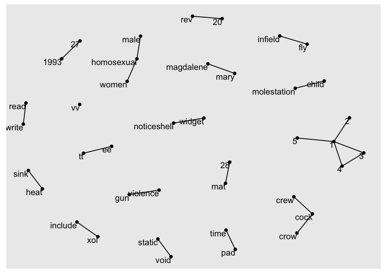
6.9 Revised version
We can improve the visualization by adding some color and some directional arrows.
a <- grid::arrow(type = "closed",
                 length = unit(.15,
                               "inches"))

ggraph(bigram_graph,
       layout = "fr") +
  geom_edge_link(aes(edge_alpha = n),
                 show.legend = FALSE,
                 arrow = a,
                 end_cap = circle(.02,
                                  'inches')) +
  geom_node_point(color = "lightblue",
                  size = 2) +
  geom_node_text(aes(label = name),
                 vjust = 1,
                 hjust = 1) +
  theme_void()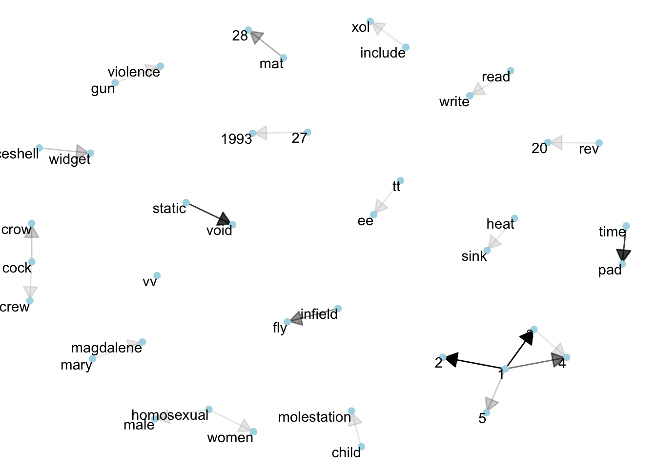
7 Reflections
This exercise exposed me for more methods of visualizing texts and the steps in doing data wrangling for text data.
Previously, I mostly was more familiar with Word Cloud. Now, tools to visualize word associations are added to my toolbox.