pacman::p_load(igraph, tidygraph, ggraph,
               visNetwork, lubridate, clock,
tidyverse, graphlayouts)Hands-on Exercise 6: Modelling, Visualising and Analysing Network Data with R
1 Overview
This hands-on exercise covers Chapter 27: Modelling, Visualising and Analysing Network Data with R.
I learned about the following:
create graph object data frames, manipulate them using appropriate functions of dplyr, lubridate, and tidygraph,
build network graph visualisation using appropriate functions of ggraph,
compute network geometrics using tidygraph,
build advanced graph visualisation by incorporating the network geometrics, and
build interactive network visualisation using visNetwork package.
2 Getting Started
2.1 Loading the required packages
For this exercise we will use the following R packages:
igraph
tidygraph
ggraph
visNetwork
tidyverse
graphlayouts
clock
2.2 Importing Data
2.2.1 About the data set
GAStech-email_edges.csv which consists of two weeks of 9063 emails correspondances between 55 employees.
This becomes the edges or lines in our network.
GAStech_email_nodes.csv which consist of the names, department and title of the 55 employees.
This becomes the nodes or points in our network.
2.2.2 Importing the data
We will import the data using read_csv.
GAStech_nodes <- read_csv("data/GAStech_email_node.csv")
GAStech_edges <- read_csv("data/GAStech_email_edge-v2.csv")
2.2.3 Initial look at the data
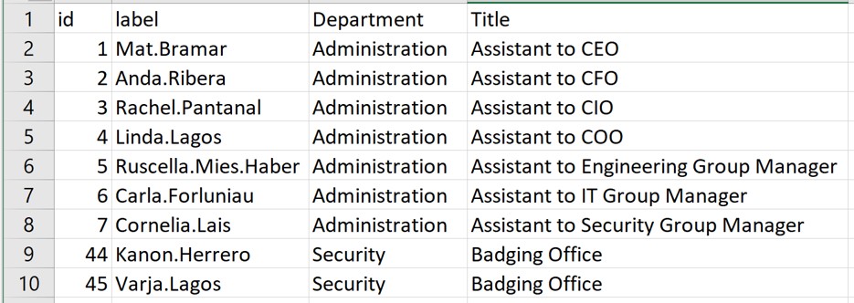
head(GAStech_nodes)# A tibble: 6 × 4
id label Department Title
<dbl> <chr> <chr> <chr>
1 1 Mat.Bramar Administration Assistant to CEO
2 2 Anda.Ribera Administration Assistant to CFO
3 3 Rachel.Pantanal Administration Assistant to CIO
4 4 Linda.Lagos Administration Assistant to COO
5 5 Ruscella.Mies.Haber Administration Assistant to Engineering Group Manag…
6 6 Carla.Forluniau Administration Assistant to IT Group Manager Contains the list of employees and their role information
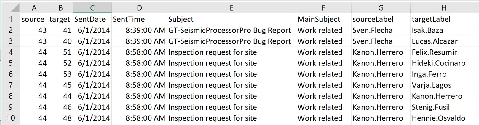
head(GAStech_edges)# A tibble: 6 × 8
source target SentDate SentTime Subject MainSubject sourceLabel targetLabel
<dbl> <dbl> <chr> <time> <chr> <chr> <chr> <chr>
1 43 41 6/1/2014 08:39 GT-Seismi… Work relat… Sven.Flecha Isak.Baza
2 43 40 6/1/2014 08:39 GT-Seismi… Work relat… Sven.Flecha Lucas.Alca…
3 44 51 6/1/2014 08:58 Inspectio… Work relat… Kanon.Herr… Felix.Resu…
4 44 52 6/1/2014 08:58 Inspectio… Work relat… Kanon.Herr… Hideki.Coc…
5 44 53 6/1/2014 08:58 Inspectio… Work relat… Kanon.Herr… Inga.Ferro
6 44 45 6/1/2014 08:58 Inspectio… Work relat… Kanon.Herr… Varja.LagosContains messages from one person to another.
3 Data Wrangling
3.1 Reviewing the edges data
glimpse(GAStech_edges)Rows: 9,063
Columns: 8
$ source <dbl> 43, 43, 44, 44, 44, 44, 44, 44, 44, 44, 44, 44, 26, 26, 26…
$ target <dbl> 41, 40, 51, 52, 53, 45, 44, 46, 48, 49, 47, 54, 27, 28, 29…
$ SentDate <chr> "6/1/2014", "6/1/2014", "6/1/2014", "6/1/2014", "6/1/2014"…
$ SentTime <time> 08:39:00, 08:39:00, 08:58:00, 08:58:00, 08:58:00, 08:58:0…
$ Subject <chr> "GT-SeismicProcessorPro Bug Report", "GT-SeismicProcessorP…
$ MainSubject <chr> "Work related", "Work related", "Work related", "Work rela…
$ sourceLabel <chr> "Sven.Flecha", "Sven.Flecha", "Kanon.Herrero", "Kanon.Herr…
$ targetLabel <chr> "Isak.Baza", "Lucas.Alcazar", "Felix.Resumir", "Hideki.Coc…3.2 Converting dates to Date datatype
We will add 2 columns to GAStech_edges, SendDate (date parse in DMY format), Weekday (what day of the week). These are generated from SentDate using lubridate functions.
GAStech_edges <- GAStech_edges %>%
  mutate(SendDate = dmy(SentDate)) %>%
  mutate(Weekday = wday(SentDate,
                        label = TRUE,
                        abbr = FALSE))
Checking GAStech_edges now have these new columns.
glimpse(GAStech_edges)Rows: 9,063
Columns: 10
$ source <dbl> 43, 43, 44, 44, 44, 44, 44, 44, 44, 44, 44, 44, 26, 26, 26…
$ target <dbl> 41, 40, 51, 52, 53, 45, 44, 46, 48, 49, 47, 54, 27, 28, 29…
$ SentDate <chr> "6/1/2014", "6/1/2014", "6/1/2014", "6/1/2014", "6/1/2014"…
$ SentTime <time> 08:39:00, 08:39:00, 08:58:00, 08:58:00, 08:58:00, 08:58:0…
$ Subject <chr> "GT-SeismicProcessorPro Bug Report", "GT-SeismicProcessorP…
$ MainSubject <chr> "Work related", "Work related", "Work related", "Work rela…
$ sourceLabel <chr> "Sven.Flecha", "Sven.Flecha", "Kanon.Herrero", "Kanon.Herr…
$ targetLabel <chr> "Isak.Baza", "Lucas.Alcazar", "Felix.Resumir", "Hideki.Coc…
$ SendDate <date> 2014-01-06, 2014-01-06, 2014-01-06, 2014-01-06, 2014-01-0…
$ Weekday <ord> Friday, Friday, Friday, Friday, Friday, Friday, Friday, Fr…3.3 Aggregating data
The edges data is not useful for network analysis as the contain individual correspondence. We instead want how many messages are sent between 2 people.
GAStech_edges_aggregated <- GAStech_edges %>%
  filter(MainSubject == "Work related") %>%
  group_by(source, target, Weekday) %>%
    summarise(Weight = n()) %>%
  filter(source!=target) %>%
  filter(Weight > 1) %>%
ungroup()glimpse(GAStech_edges_aggregated)Rows: 1,372
Columns: 4
$ source <dbl> 1, 1, 1, 1, 1, 1, 1, 1, 1, 1, 1, 1, 1, 1, 1, 1, 1, 1, 1, 1, 1,…
$ target <dbl> 2, 2, 2, 2, 2, 3, 3, 3, 3, 3, 4, 4, 4, 4, 4, 5, 5, 5, 5, 5, 6,…
$ Weekday <ord> Sunday, Monday, Tuesday, Wednesday, Friday, Sunday, Monday, Tu…
$ Weight <int> 5, 2, 3, 4, 6, 5, 2, 3, 4, 6, 5, 2, 3, 4, 6, 5, 2, 3, 4, 6, 5,…With this change we now how many messages are sent between 2 people in each day of the week. We will use this dataframe for analyzing and visualizing network data.
4 Creating network objects using tidygraph
tidygraph provides a tidy API for graph/network manipulation. While network data itself is not tidy, it can be envisioned as two tidy tables, one for node data and one for edge data. tidygraph provides a way to switch between the two tables and provides dplyr verbs for manipulating them. Furthermore it provides access to a lot of graph algorithms with return values that facilitate their use in a tidy workflow.
References:
4.1 tbl_graph object
Two functions of tidygraph package can be used to create network objects, they are:
tbl_graph()creates a tbl_graph network object from nodes and edges data.as_tbl_graph()converts network data and objects to a tbl_graph network. Below are network data and objects supported byas_tbl_graph()a node data.frame and an edge data.frame,
data.frame, list, matrix from base,
igraph from igraph,
network from network,
dendrogram and hclust from stats,
Node from data.tree,
phylo and evonet from ape, and
graphNEL, graphAM, graphBAM from graph (in Bioconductor).
4.2 The dplyr verbs in tidygraph
- activate() verb from tidygraph serves as a switch between tibbles for nodes and edges. All dplyr verbs applied to tbl_graph object are applied to the active tibble.
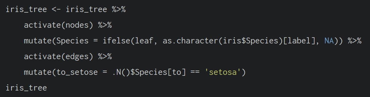
- In the above the .N() function is used to gain access to the node data while manipulating the edge data. Similarly .E() will give you the edge data and .G() will give you the tbl_graph object itself.
4.3 Using tbl_graph() to build tidygraph data model
We will use tbl_graph to build the network model:
GAStech_graph <- tbl_graph(nodes = GAStech_nodes,
                           edges = GAStech_edges_aggregated,
                           directed = TRUE)
This is a directed graph, so the direction of the messages is relevant.
4.4 Getting to know about the output
GAStech_graph# A tbl_graph: 54 nodes and 1372 edges
#
# A directed multigraph with 1 component
#
# Node Data: 54 × 4 (active)
id label Department Title
<dbl> <chr> <chr> <chr>
1 1 Mat.Bramar Administration Assistant to CEO
2 2 Anda.Ribera Administration Assistant to CFO
3 3 Rachel.Pantanal Administration Assistant to CIO
4 4 Linda.Lagos Administration Assistant to COO
5 5 Ruscella.Mies.Haber Administration Assistant to Engineering Group Mana…
6 6 Carla.Forluniau Administration Assistant to IT Group Manager
7 7 Cornelia.Lais Administration Assistant to Security Group Manager
8 44 Kanon.Herrero Security Badging Office
9 45 Varja.Lagos Security Badging Office
10 46 Stenig.Fusil Security Building Control
# ℹ 44 more rows
#
# Edge Data: 1,372 × 4
from to Weekday Weight
<int> <int> <ord> <int>
1 1 2 Sunday 5
2 1 2 Monday 2
3 1 2 Tuesday 3
# ℹ 1,369 more rowsThe output above reveals that GAStech_graph is a tbl_graph object with 54 nodes and 4541 edges.
The command also prints the first six rows of “Node Data” and the first three of “Edge Data”.
It states that the Node Data is active. The notion of an active tibble within a tbl_graph object makes it possible to manipulate the data in one tibble at a time.
4.5 Changing the active object
The nodes tibble data frame is activated by default, but you can change which tibble data frame is active with the activate() function. Thus, if we wanted to rearrange the rows in the edges tibble to list those with the highest “weight” first, we could use activate() and then arrange().
GAStech_graph %>%
  activate(edges) %>%
  arrange(desc(Weight))
# A tbl_graph: 54 nodes and 1372 edges
#
# A directed multigraph with 1 component
#
# Edge Data: 1,372 × 4 (active)
from to Weekday Weight
<int> <int> <ord> <int>
1 40 41 Saturday 13
2 41 43 Monday 11
3 35 31 Tuesday 10
4 40 41 Monday 10
5 40 43 Monday 10
6 36 32 Sunday 9
7 40 43 Saturday 9
8 41 40 Monday 9
9 19 15 Wednesday 8
10 35 38 Tuesday 8
# ℹ 1,362 more rows
#
# Node Data: 54 × 4
id label Department Title
<dbl> <chr> <chr> <chr>
1 1 Mat.Bramar Administration Assistant to CEO
2 2 Anda.Ribera Administration Assistant to CFO
3 3 Rachel.Pantanal Administration Assistant to CIO
# ℹ 51 more rows5 Plotting Static Network Graphs with ggraph package
ggraph is an extension of ggplot2, making it easier to carry over basic ggplot skills to the design of network graphs.
As in all network graph, there are three main aspects to a ggraph’s network graph, they are:
For a comprehensive discussion of each of this aspect of graph, please refer to their respective vignettes provided.
5.1 Plotting a basic network graph
The code chunk below uses ggraph(), geom-edge_link() and geom_node_point() to plot a network graph by using GAStech_graph. Before your get started, it is advisable to read their respective reference guide at least once.
ggraph(GAStech_graph) +
  geom_edge_link() +
  geom_node_point()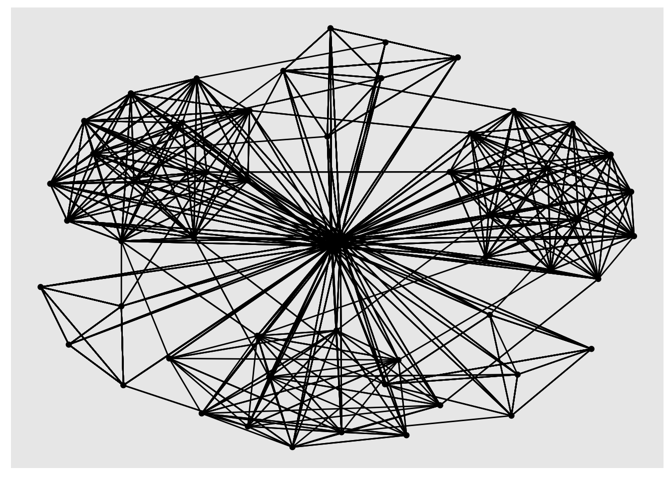
5.2 Changing the default network graph theme
n this section, you will use theme_graph() to remove the x and y axes. Before your get started, it is advisable to read it’s reference guide at least once.
g <- ggraph(GAStech_graph) +
  geom_edge_link(aes()) +
  geom_node_point(aes())

g + theme_graph()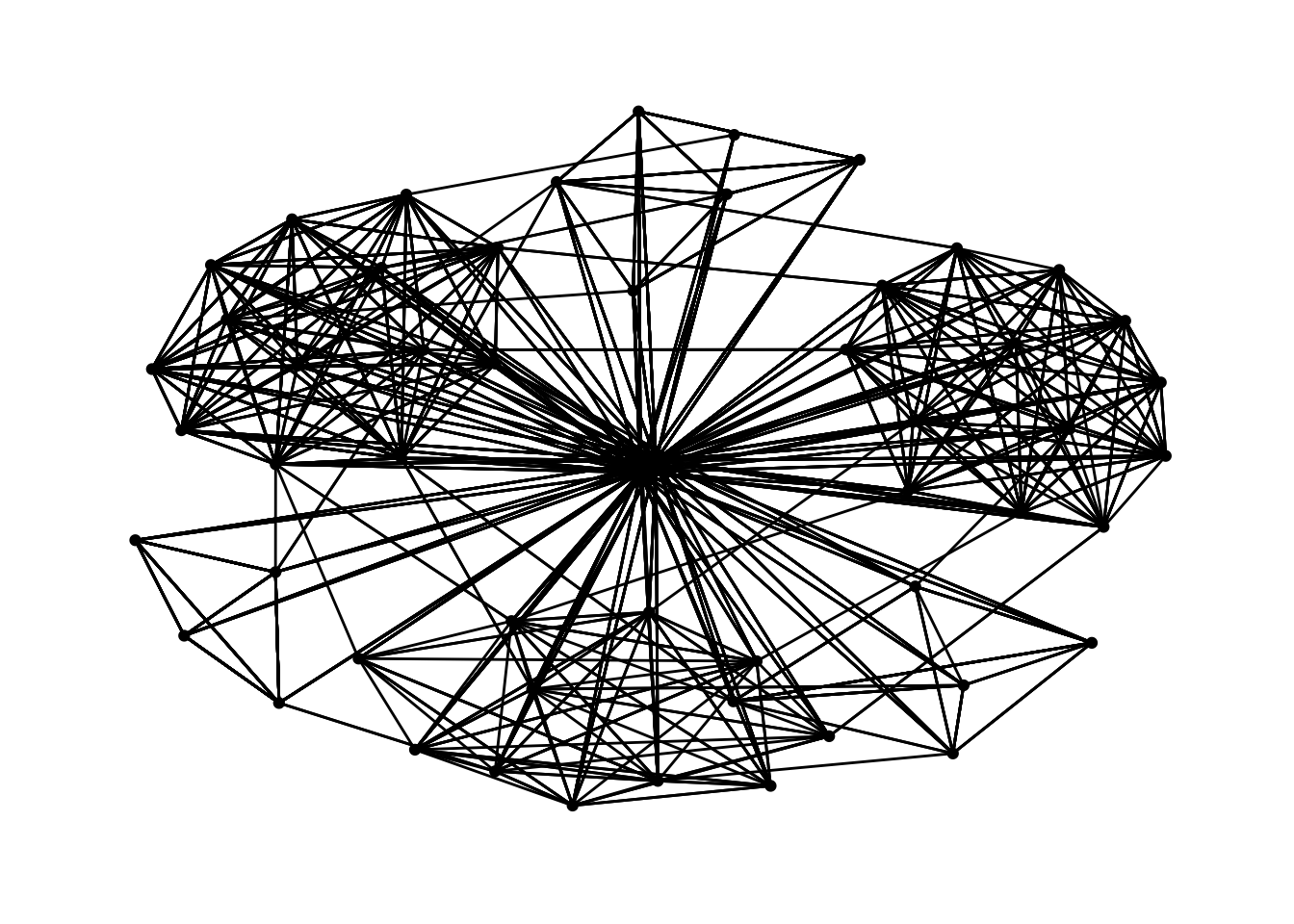
5.3 Changing the coloring of the plot
Furthermore, theme_graph() makes it easy to change the coloring of the plot.
g <- ggraph(GAStech_graph) +
  geom_edge_link(aes(colour = 'grey50')) +
  geom_node_point(aes(colour = 'grey40'))

g + theme_graph(background = 'grey10',
                text_colour = 'white')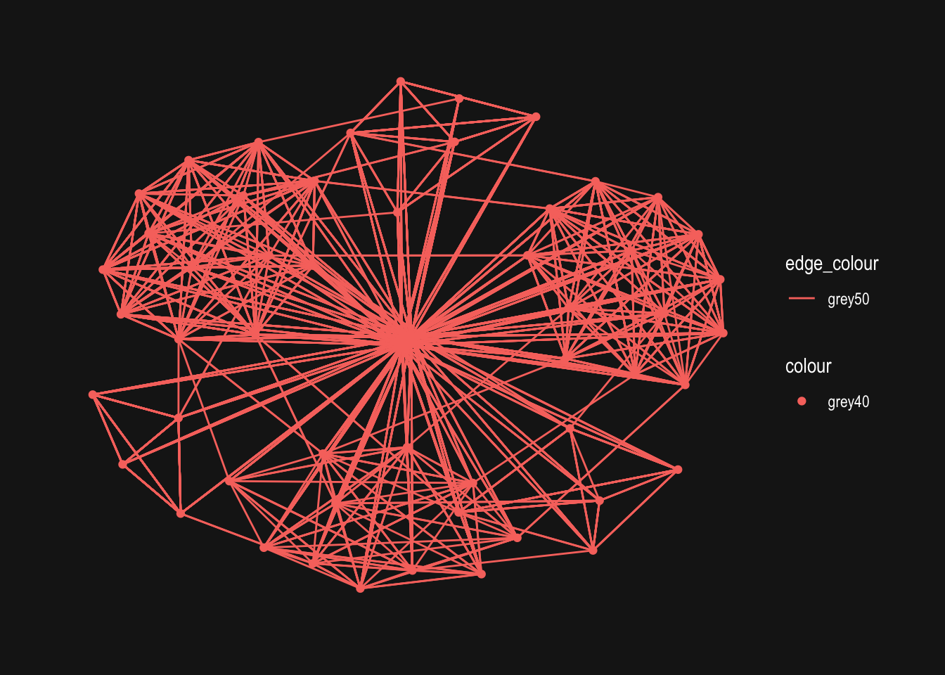
5.4 Working with ggraph’s layouts
ggraph support many layout for standard used, they are: star, circle, nicely (default), dh, gem, graphopt, grid, mds, spahere, randomly, fr, kk, drl and lgl. Figures below and on the right show layouts supported by ggraph().
5.5 Different graph layouts
The code chunks below will be used to plot the network graph using different layouts
Other documentation:
https://cran.r-project.org/web/packages/ggraph/vignettes/Layouts.html
https://ggraph.data-imaginist.com/reference/layout_tbl_graph_igraph.html
ggraph(GAStech_graph,
            layout = "fr") +
  geom_edge_link(aes()) +
  geom_node_point(aes()) +
  theme_graph()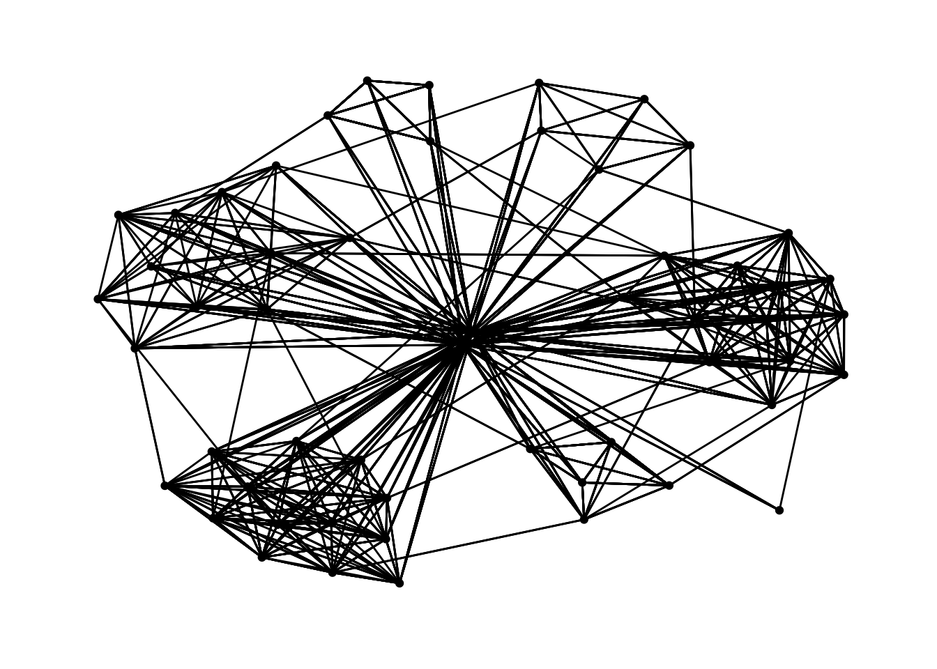
ggraph(GAStech_graph,
            layout = "nicely") +
  geom_edge_link(aes()) +
  geom_node_point(aes()) +
  theme_graph()
ggraph(GAStech_graph,
            layout = "grid") +
  geom_edge_link(aes()) +
  geom_node_point(aes()) +
  theme_graph()
ggraph(GAStech_graph,
            layout = "kk") +
  geom_edge_link(aes()) +
  geom_node_point(aes()) +
  theme_graph()
5.6 Modifying network nodes
We will color the nodes depending on the department.
ggraph(GAStech_graph,
            layout = "nicely") +
  geom_edge_link(aes()) +
  geom_node_point(aes(colour = Department,
                      size = 3)) +
  theme_graph()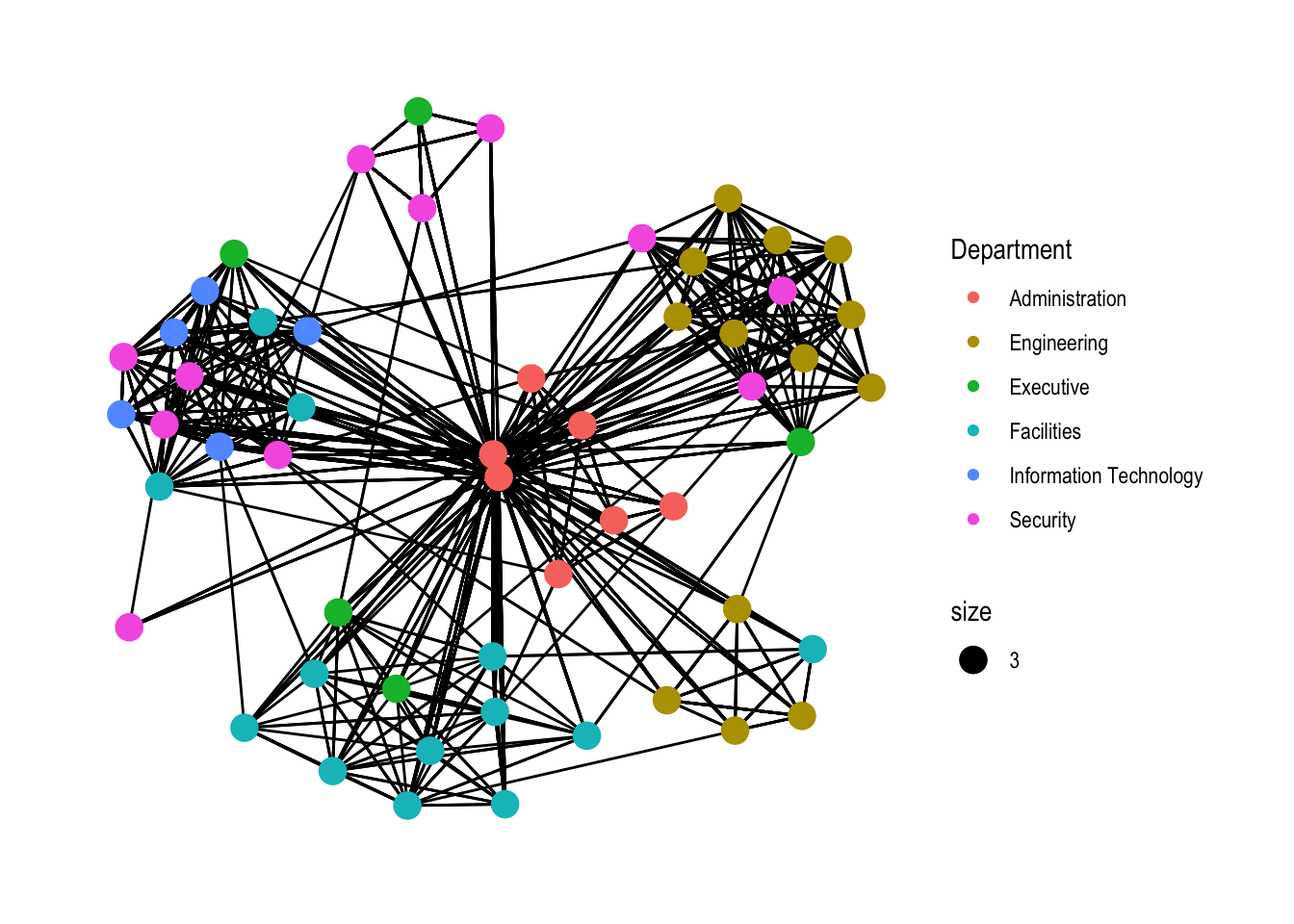
5.7 Modifiying edges
We will modify the thickness of the edges/lines based on Width.
ggraph(GAStech_graph,
            layout = "nicely") +
  geom_edge_link(aes(width=Weight),
                 alpha=0.2) +
  scale_edge_width(range = c(0.1, 5)) +
  geom_node_point(aes(colour = Department),
                  size = 3) +
  theme_graph()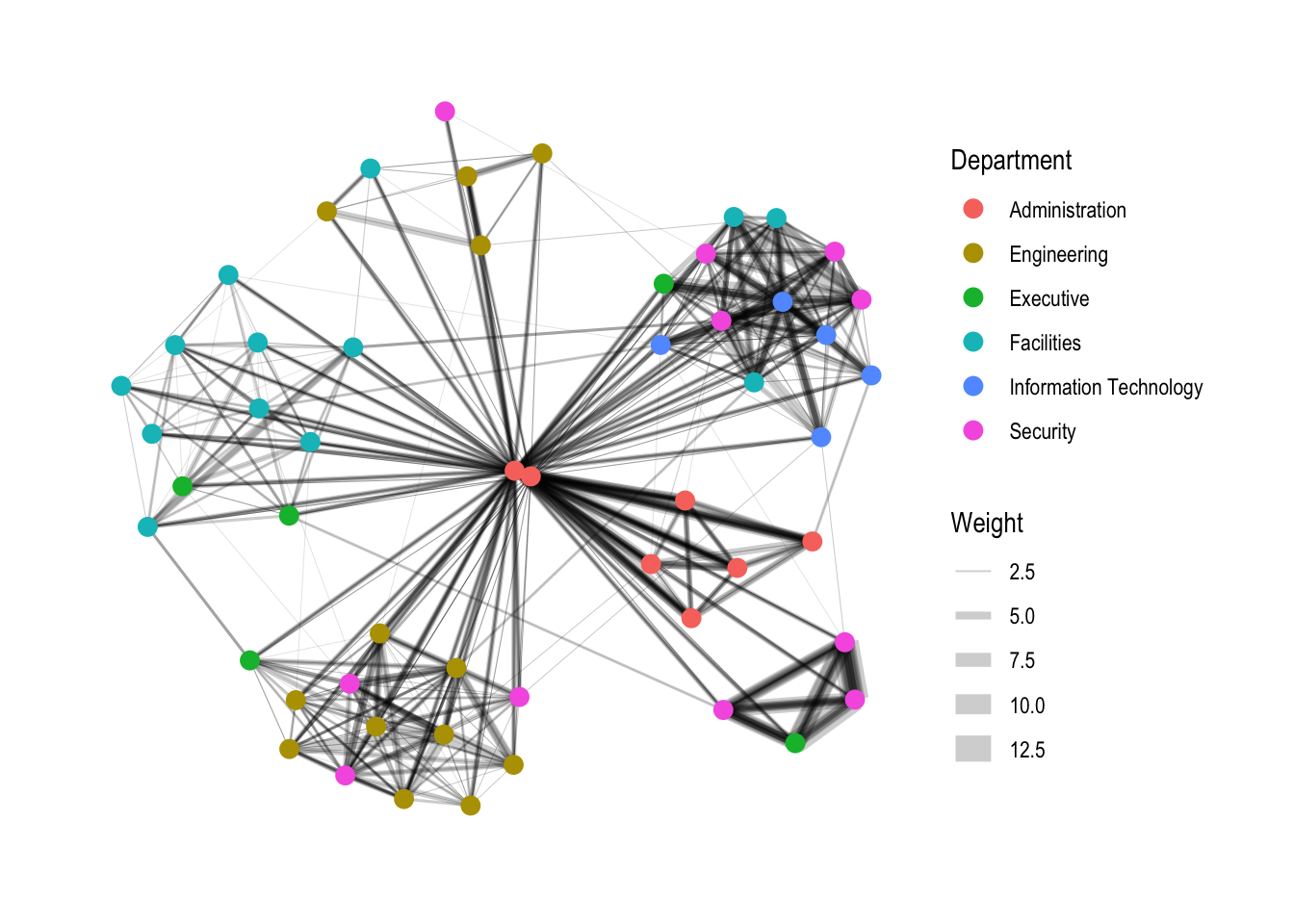
6 Creating facet graphs
Another very useful feature of ggraph is faceting. In visualising network data, this technique can be used to reduce edge over-plotting in a very meaning way by spreading nodes and edges out based on their attributes. In this section, you will learn how to use faceting technique to visualise network data.
There are three functions in ggraph to implement faceting, they are:
facet_nodes() whereby edges are only draw in a panel if both terminal nodes are present here,
facet_edges() whereby nodes are always drawn in al panels even if the node data contains an attribute named the same as the one used for the edge facetting, and
facet_graph() faceting on two variables simultaneously.
6.1 Working with facet_edges()
We can create facets for graph for each day of the week. We can do this as we have a Weekday column in our data.
set_graph_style()

ggraph(GAStech_graph,
            layout = "nicely") +
  geom_edge_link(aes(width=Weight),
                 alpha=0.2) +
  scale_edge_width(range = c(0.1, 5)) +
  geom_node_point(aes(colour = Department),
                  size = 2) +
  facet_edges(~Weekday)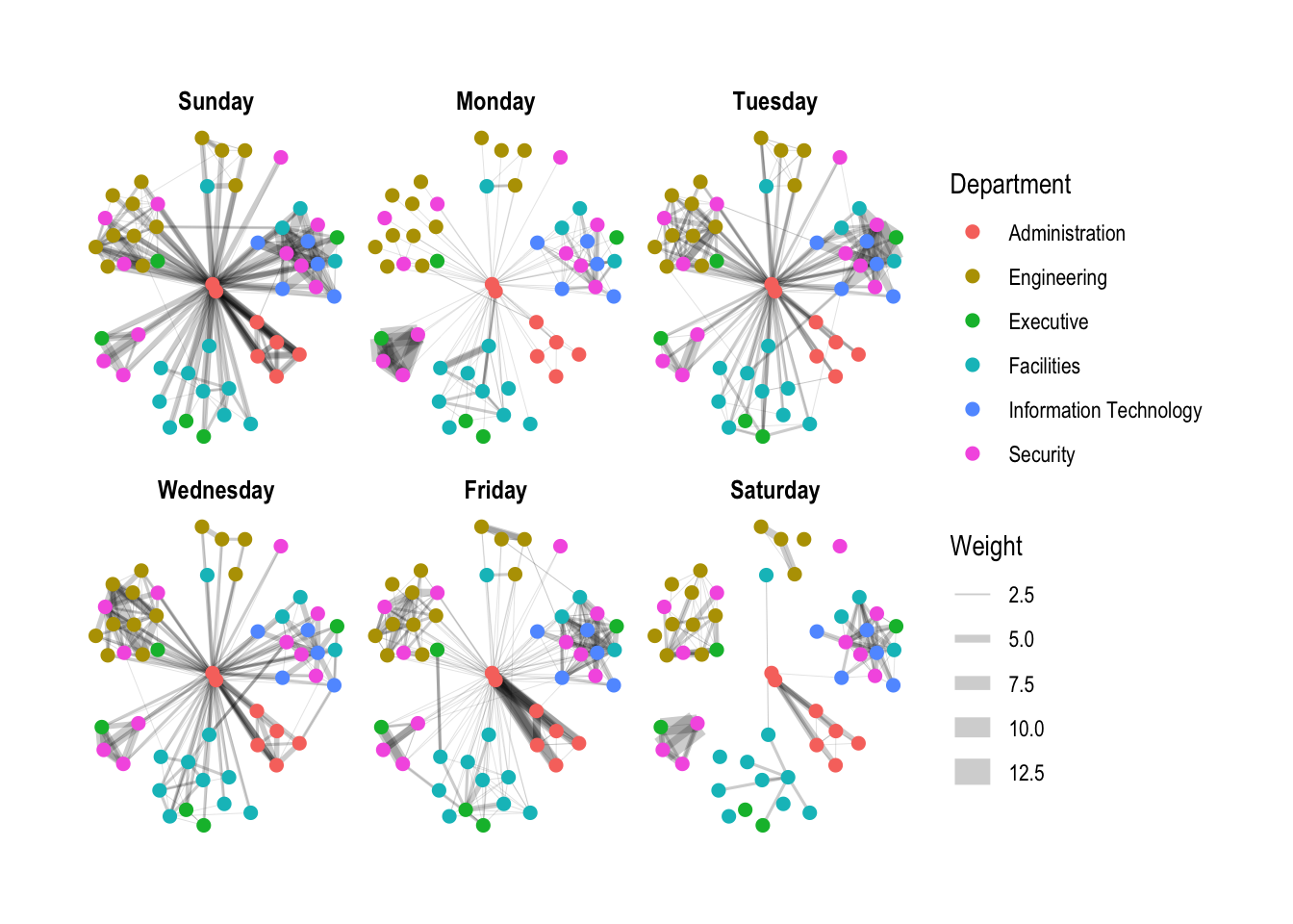
6.2 Changing the legend position
We can change the position of the legend through the theme() function.
set_graph_style()

ggraph(GAStech_graph,
            layout = "nicely") +
  geom_edge_link(aes(width=Weight),
                 alpha=0.2) +
  scale_edge_width(range = c(0.1, 5)) +
  geom_node_point(aes(colour = Department),
                  size = 2) +
  theme(legend.position = 'bottom') +
  facet_edges(~Weekday)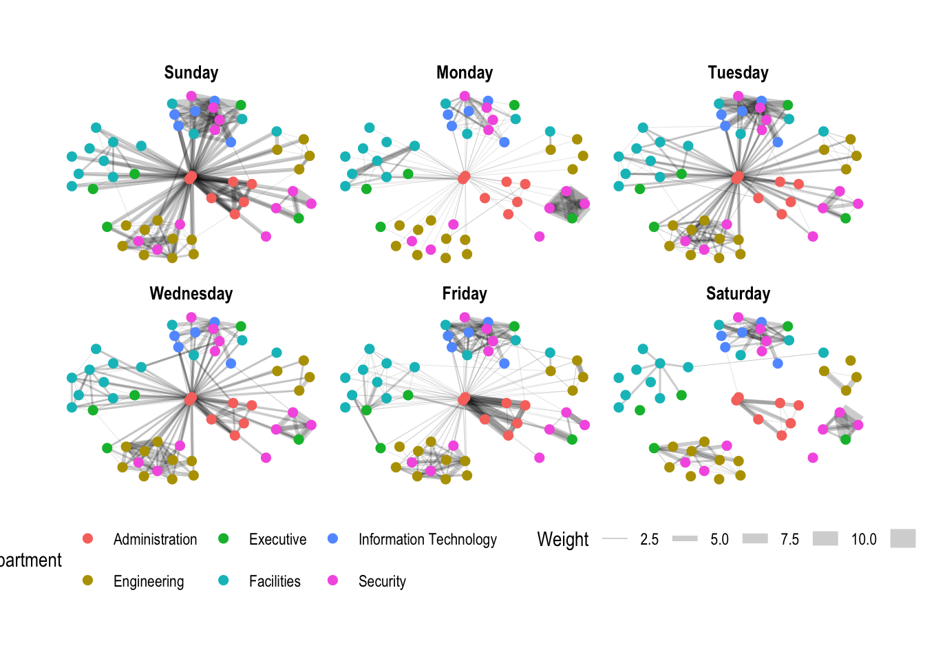
6.3 Adding frame to each facet
We can also add frames to each facet.
set_graph_style()

ggraph(GAStech_graph,
            layout = "nicely") +
  geom_edge_link(aes(width=Weight),
                 alpha=0.2) +
  scale_edge_width(range = c(0.1, 5)) +
  geom_node_point(aes(colour = Department),
                  size = 2) + facet_edges(~Weekday) +
  th_foreground(foreground = "grey80",
                border = TRUE) +
  theme(legend.position = 'bottom')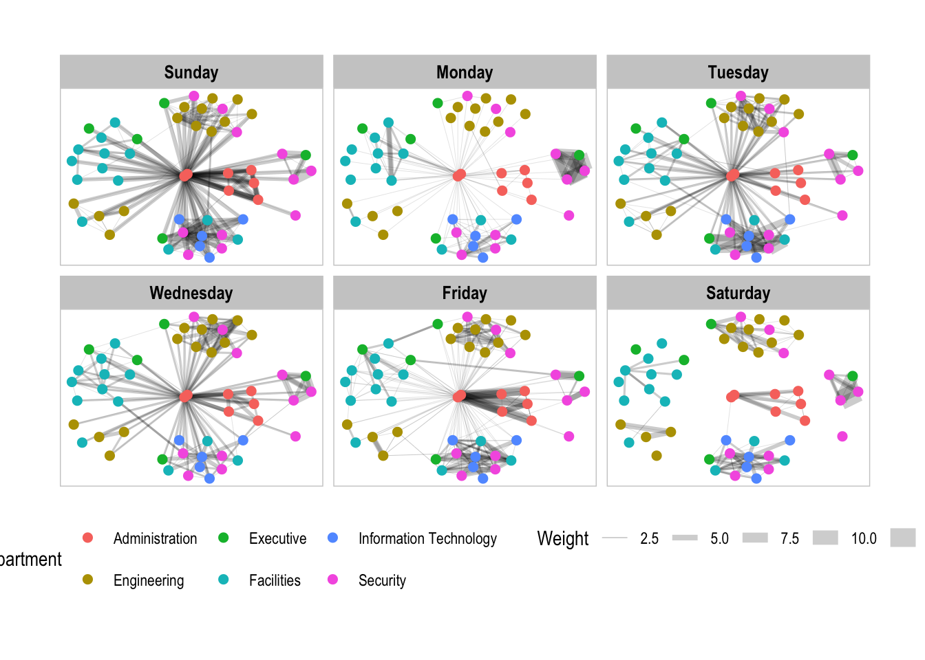
6.4 Working with facet_nodes()
We can also facet by nodes. In our case, let’s try to facet by Department.
set_graph_style()

ggraph(GAStech_graph,
            layout = "nicely") +
  geom_edge_link(aes(width=Weight),
                 alpha=0.2) +
  scale_edge_width(range = c(0.1, 5)) +
  geom_node_point(aes(colour = Department),
                  size = 2) +
  facet_nodes(~Department)+
  th_foreground(foreground = "grey80",
                border = TRUE) +
  theme(legend.position = 'bottom')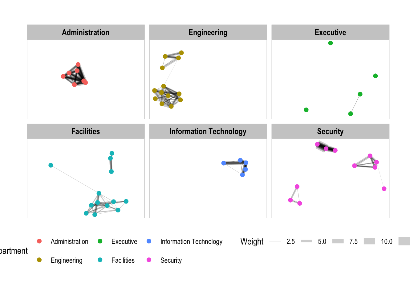
7 Network Metrics Analysis
7.1 Computing centrality indices
Centrality measures are a collection of statistical indices use to describe the relative important of the actors are to a network. There are four well-known centrality measures, namely: degree, betweenness, closeness and eigenvector. It is beyond the scope of this hands-on exercise to cover the principles and mathematics of these measure here.
GAStech_graph %>%
  mutate(betweenness_centrality = centrality_betweenness()) %>%
  ggraph(layout = "fr") +
  geom_edge_link(aes(width=Weight),
                 alpha=0.2) +
  scale_edge_width(range = c(0.1, 5)) +
  geom_node_point(aes(colour = Department,
            size=betweenness_centrality), alpha = 0.8) +
  theme_graph()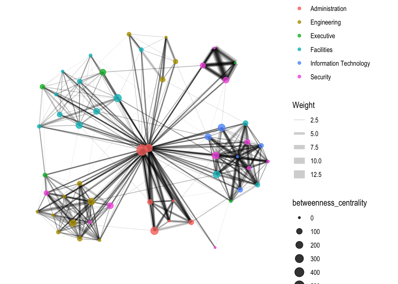
7.2 Visualising network metrics
We can also compute the central tendency from ggraph itself, without pre-computing like when we added betweenness_centrality column above.
GAStech_graph %>%
  ggraph(layout = "fr") +
  geom_edge_link(aes(width=Weight),
                 alpha=0.2) +
  scale_edge_width(range = c(0.1, 5)) +
  geom_node_point(aes(colour = Department,
                      size = centrality_betweenness())) +
  theme_graph()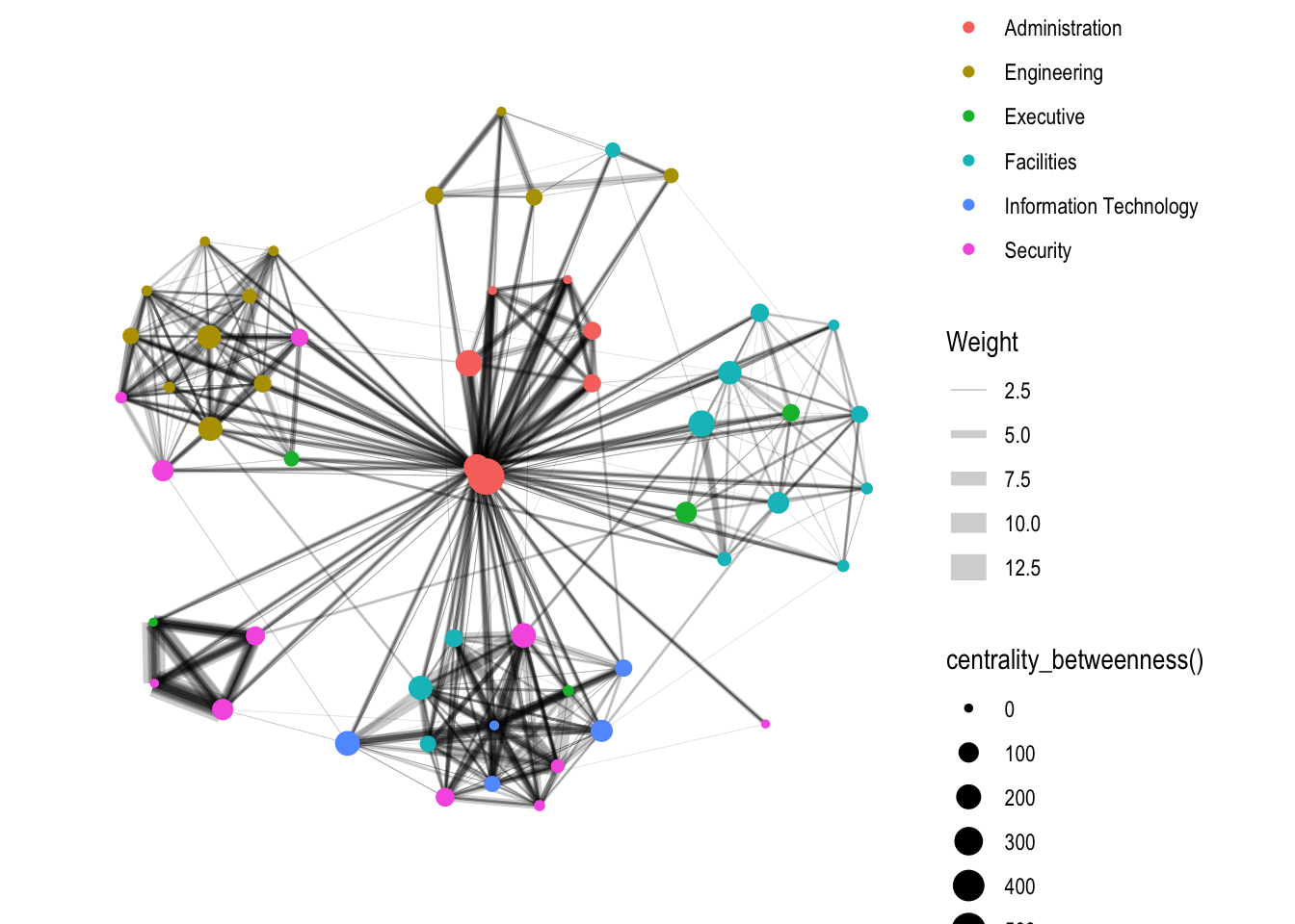
7.3 Visualising Community
Communities are a group of nodes that are closely-knit. The measure of being closely-knit is the Weight column in our graph.
Other references: https://towardsdatascience.com/community-detection-algorithms-9bd8951e7dae
GAStech_graph %>%
  mutate(community = as.factor(group_edge_betweenness(weights = Weight, directed = TRUE))) %>%
  ggraph(layout = "fr") +
  geom_edge_link(aes(width=Weight),
                 alpha=0.2) +
  scale_edge_width(range = c(0.1, 5)) +
  geom_node_point(aes(colour = community)) +
  theme_graph()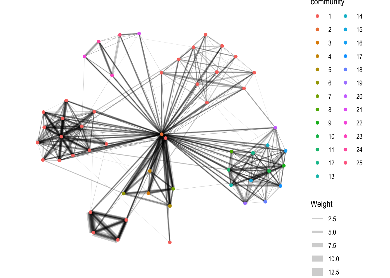
8 Building interactive network graph with visNetwork
8.1 Data preparation
Before we can plot the interactive network graph, we need to prepare the data model. We will add the labels to the nodes in the edge graph. This is why we will join the edge and node dataframes.
GAStech_edges_aggregated <- GAStech_edges %>%
  left_join(GAStech_nodes, by = c("sourceLabel" = "label")) %>%
  rename(from = id) %>%
  left_join(GAStech_nodes, by = c("targetLabel" = "label")) %>%
  rename(to = id) %>%
  filter(MainSubject == "Work related") %>%
  group_by(from, to) %>%
    summarise(weight = n()) %>%
  filter(from!=to) %>%
  filter(weight > 1) %>%
  ungroup()
8.2 Plotting the first interactive network graph
visNetwork(GAStech_nodes,
           GAStech_edges_aggregated)
8.3 Working with layout
We can also change the layout of the interactive graph. In this example, Fruchterman and Reingold layout is used.
visNetwork(GAStech_nodes,
           GAStech_edges_aggregated) %>%
visIgraphLayout(layout = "layout_with_fr") 8.4 Working with visual attributes - Nodes
visNetwork() looks for a field called “group” in the nodes object and colour the nodes according to the values of the group field.
We will create a group column from Department.
GAStech_nodes <- GAStech_nodes %>%
  mutate(group = Department)
After adding the group column, we can replot.
visNetwork(GAStech_nodes,
           GAStech_edges_aggregated) %>%
  visIgraphLayout(layout = "layout_with_fr") %>%
  visLegend() %>%
  visLayout(randomSeed = 123)
8.5 Working with visual attributes - Edges
In the code run below visEdges() is used to symbolise the edges.
- The argument arrows is used to define where to place the arrow.
- The smooth argument is used to plot the edges using a smooth curve.
visNetwork(GAStech_nodes,
           GAStech_edges_aggregated) %>%
  visIgraphLayout(layout = "layout_with_fr") %>%
  visEdges(arrows = "to",
           smooth = list(enabled = TRUE,
                         type = "curvedCW")) %>%
  visLegend() %>%
  visLayout(randomSeed = 123)
8.6 Adding Interactivity
In the code chunk below, visOptions() is used to incorporate interactivity features in the data visualisation.
The argument highlightNearest highlights nearest when clicking a node.
The argument nodesIdSelection adds an id node selection creating an HTML select element.
visNetwork(GAStech_nodes,
           GAStech_edges_aggregated) %>%
  visIgraphLayout(layout = "layout_with_fr") %>%
  visOptions(highlightNearest = TRUE,
             nodesIdSelection = TRUE) %>%
  visLegend() %>%
  visLayout(randomSeed = 123)
9 Reflections
This exercise is one of the most interesting for me as I have been plotting network graphs for my personal project before (using Javascript).
It was eye-opening to know that there are different layouts that can be used. I always thought they are randomly-generated.