In-class Exercise 6A: Visualising and Analysing Network Data

1 Overview

We will visualize and analyze text data using King James Bible

ref: https://kgjerde.github.io/corporaexplorer/articles/bible.html

2 Getting Started

2.1 Loading the required packages

pacman::p_load(jsonlite, tidygraph, ggraph, visNetwork, graphlayouts, ggforce, skimr, tidytext, tidyverse)

2.2 Loading the data

mc3_data <- fromJSON("data/MC3.json")

class(mc3_data)

[1] "list"

3 Extracting network elements

3.1 Extracting edges

mc3_edges <-
  as_tibble(mc3_data$links) %>%
  distinct() %>%
  mutate(
    source = as.character(source),
    target=as.character(target),
    type = as.character(type)
  ) %>%
  group_by(source, target, type) %>%
  summarize(weights = n()) %>%
  filter(source!=target) %>%
  ungroup()

3.2 Extracting nodes

mc3_nodes <- as_tibble(mc3_data$nodes) %>%
  mutate(
    country = as.character(country),
    id = as.character(id),
    product_services = as.character(product_services),
    revenue_omu = as.numeric(as.character(revenue_omu)),
    type = as.character(type)
  ) %>%
  select(id, country, type, revenue_omu, product_services)

id1 <- mc3_edges %>%
  select(source) %>%
  rename(id = source)
id2 <- mc3_edges %>%
  select(target) %>%
  rename(id = target)
mc3_nodes1 <- rbind(id1, id2) %>%
  distinct() %>%
  left_join(mc3_nodes,
            unmatched = "drop")

mc3_graph <- tbl_graph(nodes = mc3_nodes1,
                       edges = mc3_edges,
                       directed = FALSE) %>%
  mutate(
    betweenness_centrality = centrality_betweenness(),
    close_centrality = centrality_closeness()
  )

We calculated edge weights. However, since centrality calculations are undirected, the weights are not relevant.

It only matters if the nodes are connected or not.

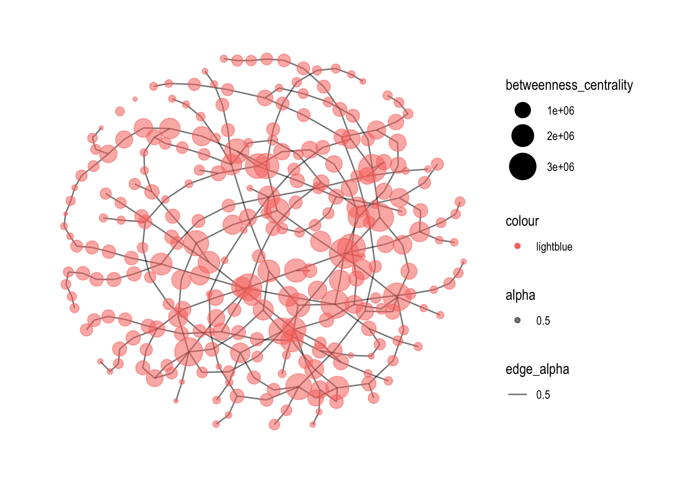
mc3_graph %>%
  filter(betweenness_centrality >= 300000) %>%
  ggraph(layout = "fr") +
  geom_edge_link(aes(alpha = 0.5)) +
  geom_node_point(aes(
    size = betweenness_centrality,
    color = "lightblue",
    alpha = 0.5
  )) +
  scale_size_continuous(range=c(1,10))+
  theme_graph()