Hands-on Exercise 9E: Treemap Visualisation with R

Author

Kristine Joy Paas

Published

June 13, 2024

Modified

June 13, 2024

1 Overview

This hands-on exercise covers Chapter 16: Treemap Visualisation with R.

In this exercise, I learned:

Creating Treemap Visualizations

2 Getting Started

2.1 Loading the required packages

For this exercise we will use the following R packages:

pacman::p_load(treemap, treemapify, tidyverse)

2.2 Importing data

In this exercise, REALIS2018.csv data will be used. This dataset provides information of private property transaction records in 2018. The dataset is extracted from REALIS portal (https://spring.ura.gov.sg/lad/ore/login/index.cfm) of Urban Redevelopment Authority (URA).

realis2018 <- read_csv("data/realis2018.csv")

glimpse(realis2018)

Rows: 23,205
Columns: 20
$ `Project Name`                <chr> "ADANA @ THOMSON", "ALANA", "ALANA", "AL…
$ Address                       <chr> "8 Old Upper Thomson Road  #05-03", "156…
$ `No. of Units`                <dbl> 1, 1, 1, 1, 1, 1, 1, 1, 1, 1, 1, 1, 1, 1…
$ `Area (sqm)`                  <dbl> 52, 284, 256, 256, 277, 285, 234, 155, 1…
$ `Type of Area`                <chr> "Strata", "Strata", "Strata", "Strata", …
$ `Transacted Price ($)`        <dbl> 888888, 2530000, 2390863, 2450000, 19800…
$ `Nett Price($)`               <chr> "-", "-", "2382517", "2441654", "-", "-"…
$ `Unit Price ($ psm)`          <dbl> 17094, 8908, 9307, 9538, 7148, 6947, 147…
$ `Unit Price ($ psf)`          <dbl> 1588, 828, 865, 886, 664, 645, 1371, 149…
$ `Sale Date`                   <chr> "4-Jul-18", "5-Oct-18", "9-Jun-18", "14-…
$ `Property Type`               <chr> "Apartment", "Terrace House", "Terrace H…
$ Tenure                        <chr> "Freehold", "103 Yrs From 12/08/2013", "…
$ `Completion Date`             <chr> "2018", "2018", "2018", "2018", "2008", …
$ `Type of Sale`                <chr> "New Sale", "Sub Sale", "New Sale", "New…
$ `Purchaser Address Indicator` <chr> "Private", "Private", "HDB", "N.A", "Pri…
$ `Postal District`             <dbl> 20, 28, 28, 28, 26, 26, 26, 26, 26, 26, …
$ `Postal Sector`               <dbl> 57, 80, 80, 80, 78, 78, 78, 78, 78, 78, …
$ `Postal Code`                 <dbl> 573868, 804555, 804529, 804540, 786300, …
$ `Planning Region`             <chr> "North East Region", "North East Region"…
$ `Planning Area`               <chr> "Ang Mo Kio", "Ang Mo Kio", "Ang Mo Kio"…

3 Data Wrangling

This dataset contains information about individual transactions. For our visualization, we will aggregate the transactions as treemap visualization is used for visualization aggregated data.

We will aggregate by:

Project Name
Planning Region
Planning Area
Property Type
Type of Sale

realis2018_summarised <- realis2018 %>% 
  group_by(`Project Name`,`Planning Region`, 
           `Planning Area`, `Property Type`, 
           `Type of Sale`) %>%
  summarise(`Total Unit Sold` = sum(`No. of Units`, na.rm = TRUE), 
            `Total Area` = sum(`Area (sqm)`, na.rm = TRUE),
            `Median Unit Price ($ psm)` = median(`Unit Price ($ psm)`, na.rm = TRUE),
            `Median Transacted Price` = median(`Transacted Price ($)`, na.rm = TRUE))

4 Designing Treemap with with treemap Package

4.1 Designing a static treemap

We will first filter Resale records for Condominiums.

realis2018_selected <- realis2018_summarised %>%
  filter(`Property Type` == "Condominium", `Type of Sale` == "Resale")

4.2 Using basic arguments

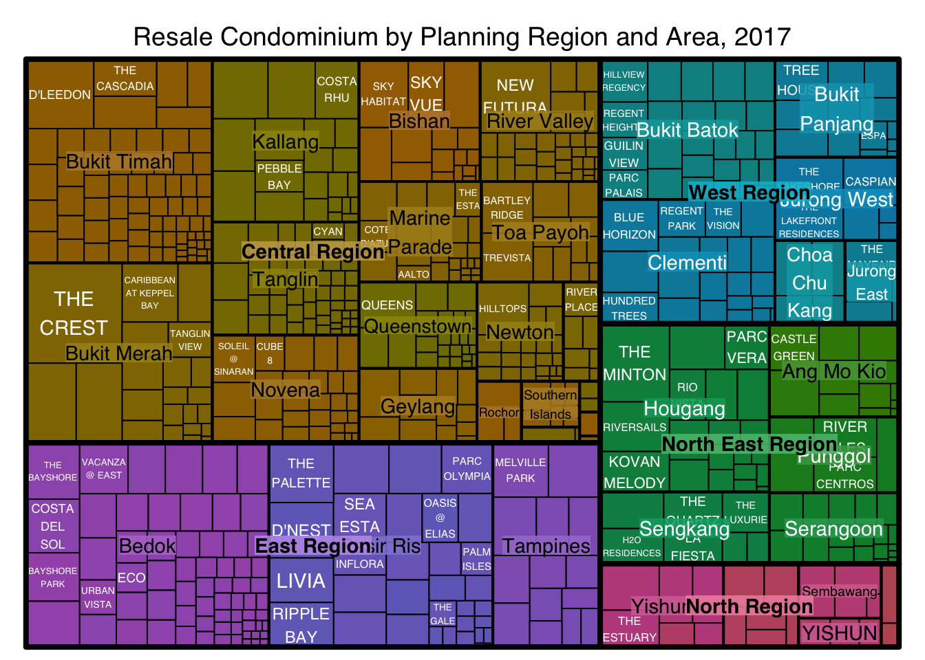
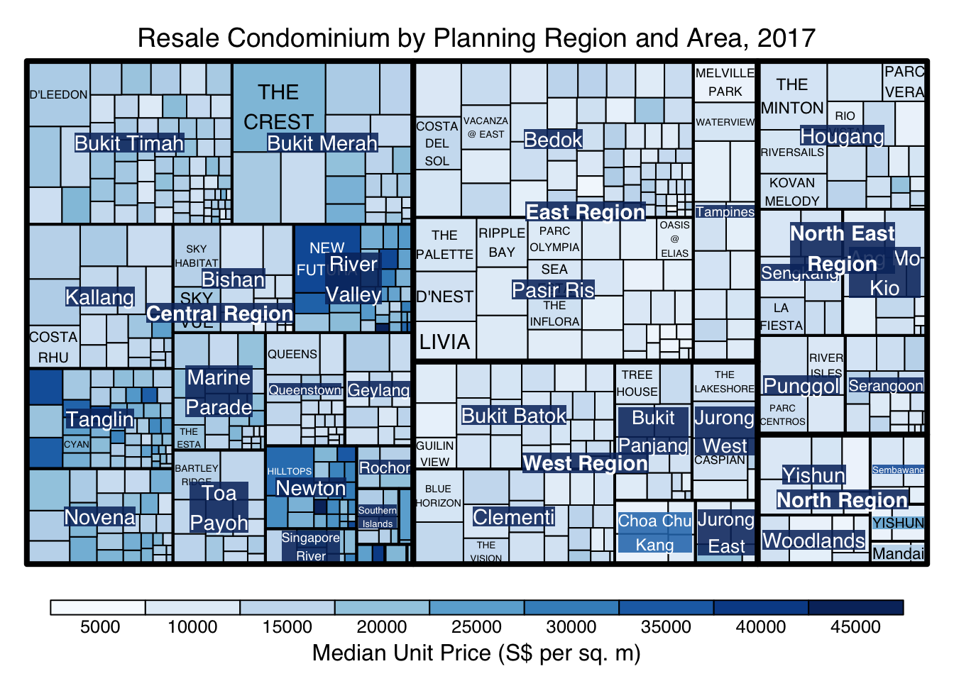
The code chunk below designed a treemap by using three core arguments of treemap(), namely: index, vSize and vColor.

treemap(realis2018_selected,
        index=c("Planning Region", "Planning Area", "Project Name"),
        vSize="Total Unit Sold",
        vColor="Median Unit Price ($ psm)",
        title="Resale Condominium by Planning Region and Area, 2017",
        title.legend = "Median Unit Price (S$ per sq. m)"
        )

4.3 Working with vcolor and type arguments

We will attach the color to the Median unit price. This is so we have information on both:

area = total units sold
color = median price

treemap(realis2018_selected,
        index=c("Planning Region", "Planning Area", "Project Name"),
        vSize="Total Unit Sold",
        vColor="Median Unit Price ($ psm)",
        type = "value",
        title="Resale Condominium by Planning Region and Area, 2017",
        title.legend = "Median Unit Price (S$ per sq. m)"
        )

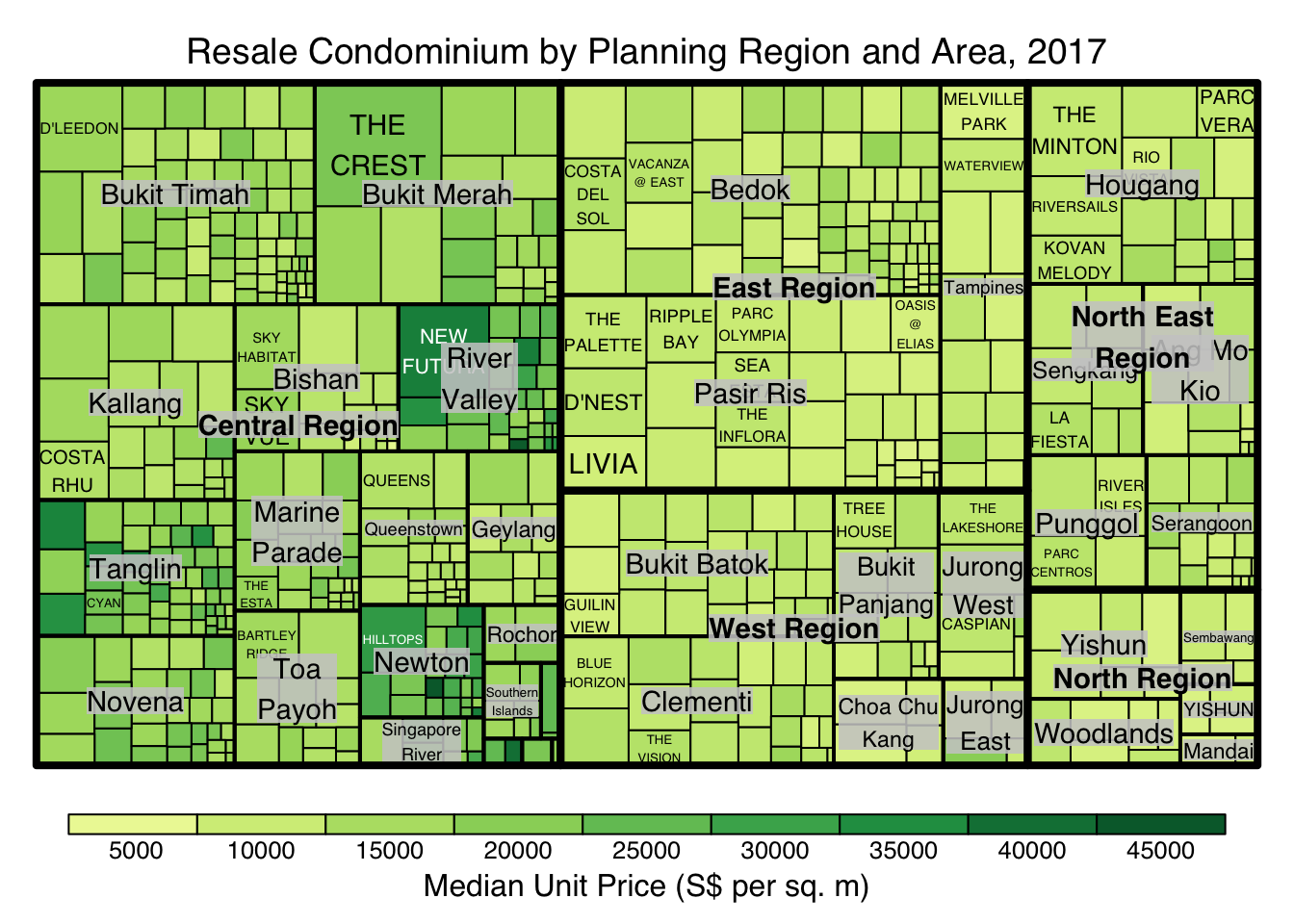
4.4 The value type treemap

treemap(realis2018_selected,
        index=c("Planning Region", "Planning Area", "Project Name"),
        vSize="Total Unit Sold",
        vColor="Median Unit Price ($ psm)",
        type="value",
        palette="RdYlBu", 
        title="Resale Condominium by Planning Region and Area, 2017",
        title.legend = "Median Unit Price (S$ per sq. m)"
        )

This uses a diverging palette (RdYlBu) even if there are no negative values so the Reds are not untilized.

4.5 The manual type treemap

manual maps the values to the full color range.

treemap(realis2018_selected,
        index=c("Planning Region", "Planning Area", "Project Name"),
        vSize="Total Unit Sold",
        vColor="Median Unit Price ($ psm)",
        type="manual",
        palette="RdYlBu", 
        title="Resale Condominium by Planning Region and Area, 2017",
        title.legend = "Median Unit Price (S$ per sq. m)"
        )

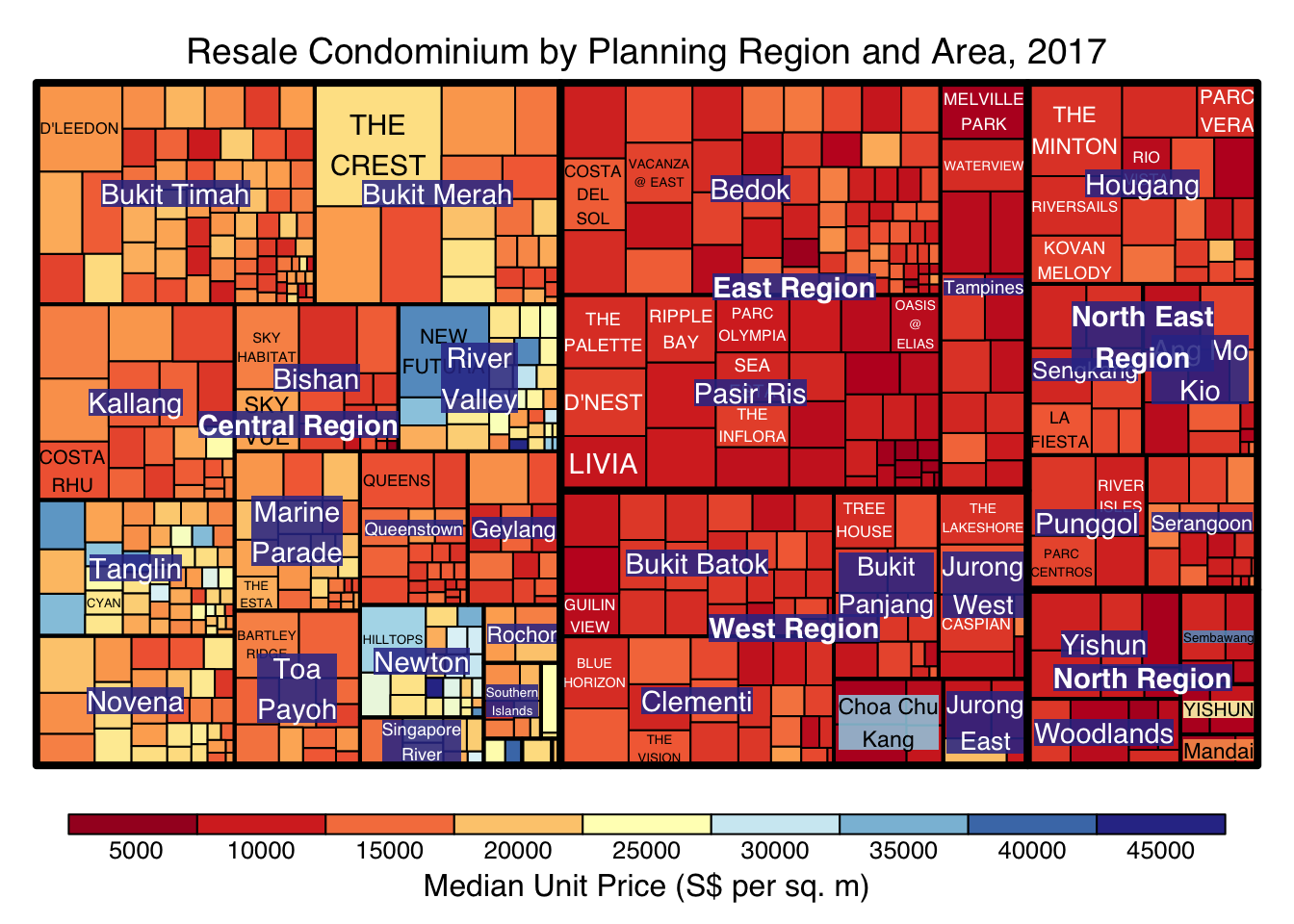
As previously mentioned, this uses a diverging palette (RdYlBu) and the current visualization is confusing as cheapest properties map to Red, which is usually perceived as negative.

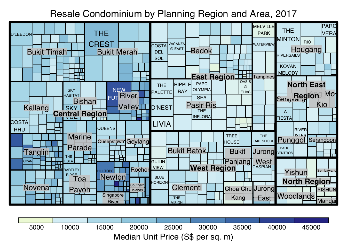
It is better to use a single color palette as we have no negative prices anyway.

treemap(realis2018_selected,
        index=c("Planning Region", "Planning Area", "Project Name"),
        vSize="Total Unit Sold",
        vColor="Median Unit Price ($ psm)",
        type="manual",
        palette="Blues", 
        title="Resale Condominium by Planning Region and Area, 2017",
        title.legend = "Median Unit Price (S$ per sq. m)"
        )

4.6 Treemap Layout

treemap() supports two popular treemap layouts, namely: “squarified” and “pivotSize”. The default is “pivotSize”.

The squarified treemap algorithm (Bruls et al., 2000) produces good aspect ratios, but ignores the sorting order of the rectangles (sortID). The ordered treemap, pivot-by-size, algorithm (Bederson et al., 2002) takes the sorting order (sortID) into account while aspect ratios are still acceptable.

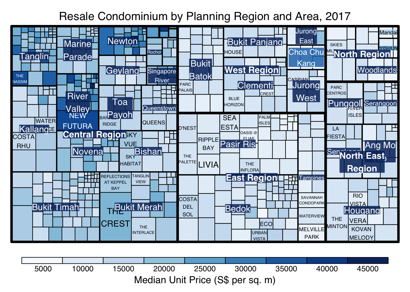
4.7 Working with algorithm argument

The code chunk below plots a squarified treemap by changing the algorithm argument.

treemap(realis2018_selected,
        index=c("Planning Region", "Planning Area", "Project Name"),
        vSize="Total Unit Sold",
        vColor="Median Unit Price ($ psm)",
        type="manual",
        palette="Blues", 
        algorithm = "squarified",
        title="Resale Condominium by Planning Region and Area, 2017",
        title.legend = "Median Unit Price (S$ per sq. m)"
        )

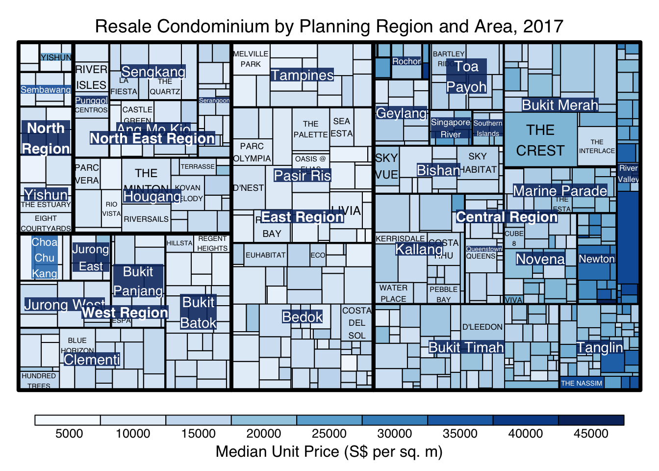
4.8 Using sortID

When “pivotSize” algorithm is used, sortID argument can be used to dertemine the order in which the rectangles are placed from top left to bottom right.

treemap(realis2018_selected,
        index=c("Planning Region", "Planning Area", "Project Name"),
        vSize="Total Unit Sold",
        vColor="Median Unit Price ($ psm)",
        type="manual",
        palette="Blues", 
        algorithm = "pivotSize",
        sortID = "Median Transacted Price",
        title="Resale Condominium by Planning Region and Area, 2017",
        title.legend = "Median Unit Price (S$ per sq. m)"
        )

5 Designing a Treemap using treemapify Package

treemapify is a R package specially developed to draw treemaps in ggplot2.

5.1 Designing a basic treemap

ggplot(data=realis2018_selected, 
       aes(area = `Total Unit Sold`,
           fill = `Median Unit Price ($ psm)`),
       layout = "scol",
       start = "bottomleft") + 
  geom_treemap() +
  scale_fill_gradient(low = "light blue", high = "blue")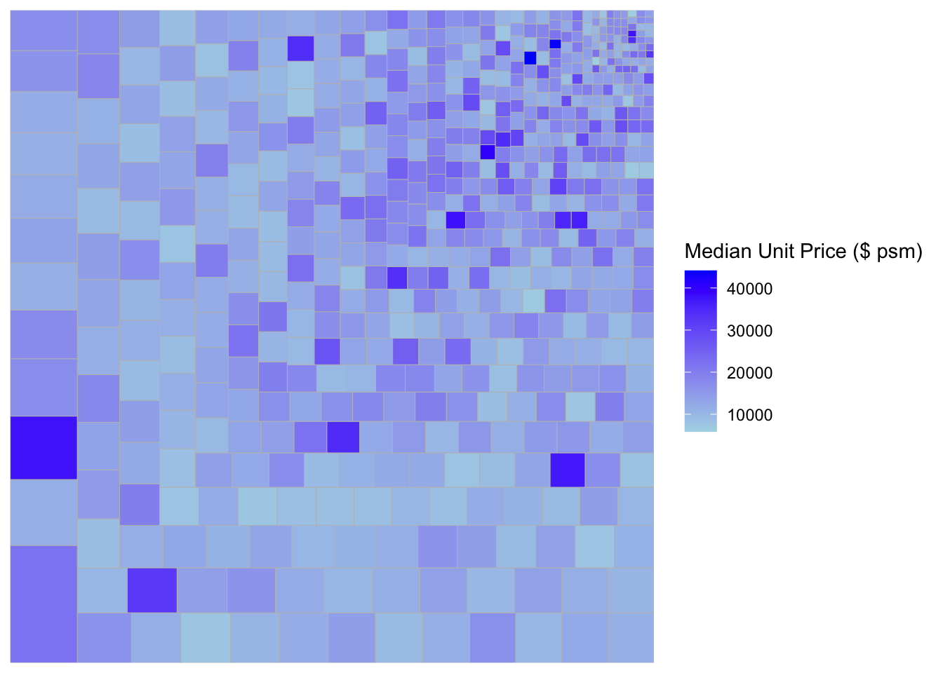

5.2 Defining hierarchy

We can group by planning region.

ggplot(data=realis2018_selected, 
       aes(area = `Total Unit Sold`,
           fill = `Median Unit Price ($ psm)`,
           subgroup = `Planning Region`),
       start = "topleft") + 
  geom_treemap()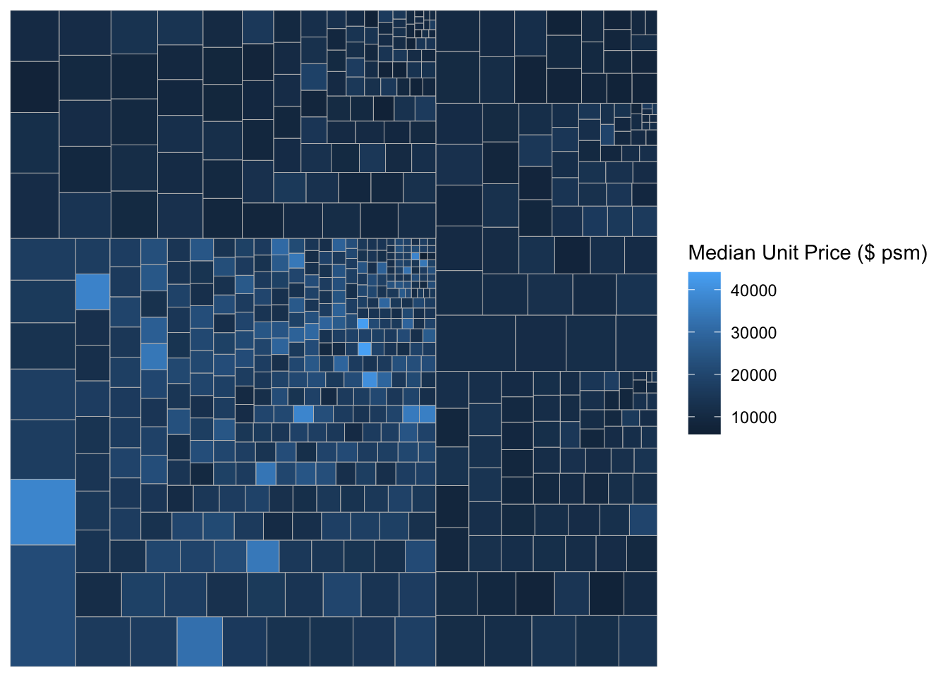

Similarly, we can also group by planning area, or other variables.

ggplot(data=realis2018_selected, 
       aes(area = `Total Unit Sold`,
           fill = `Median Unit Price ($ psm)`,
           subgroup = `Planning Region`,
           subgroup2 = `Planning Area`)) + 
  geom_treemap()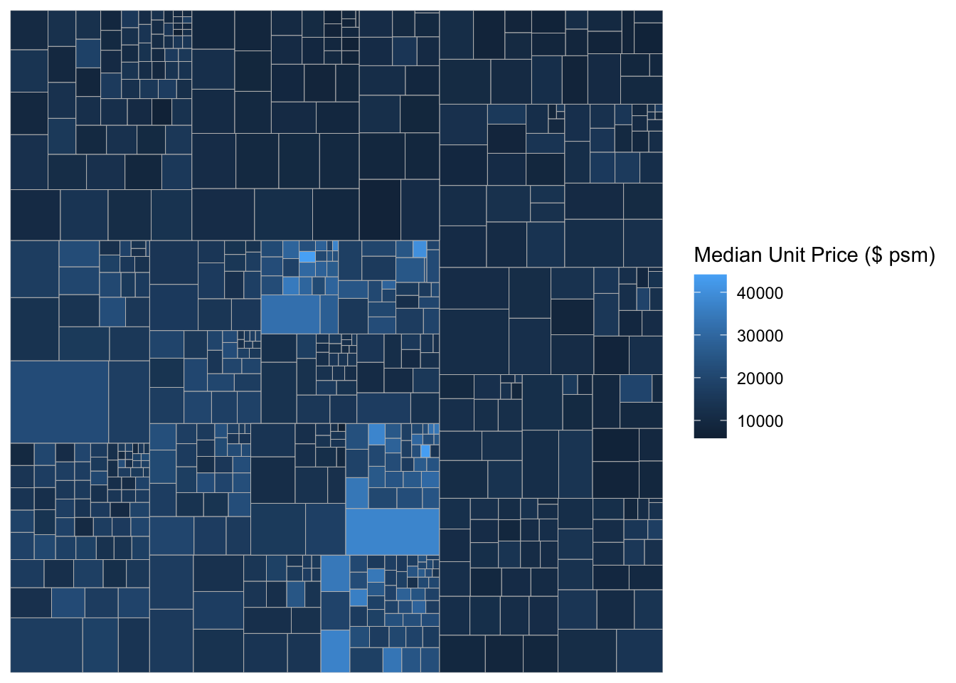

We can also have boundary lines to separate the areas better.

ggplot(data=realis2018_selected, 
       aes(area = `Total Unit Sold`,
           fill = `Median Unit Price ($ psm)`,
           subgroup = `Planning Region`,
           subgroup2 = `Planning Area`)) + 
  geom_treemap() +
  geom_treemap_subgroup2_border(colour = "gray40",
                                size = 2) +
  geom_treemap_subgroup_border(colour = "gray20")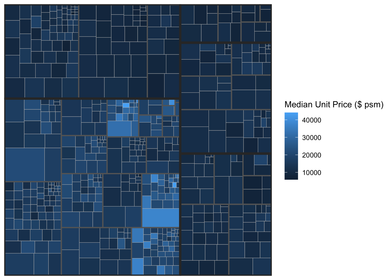

6 Designing Interactive Treemap using d3treeR

6.1 Installing d3treeR package

d3treeR is not on CRAN so we have to take a different route in installing.

install.packages("devtools")

library(devtools)
install_github("timelyportfolio/d3treeR")

library(d3treeR)

6.2 Designing an Interactive Treemap

treemap() is used to generate a static treemap.

tm <- treemap(realis2018_summarised,
        index=c("Planning Region", "Planning Area"),
        vSize="Total Unit Sold",
        vColor="Median Unit Price ($ psm)",
        type="value",
        title="Private Residential Property Sold, 2017",
        title.legend = "Median Unit Price (S$ per sq. m)"
        )

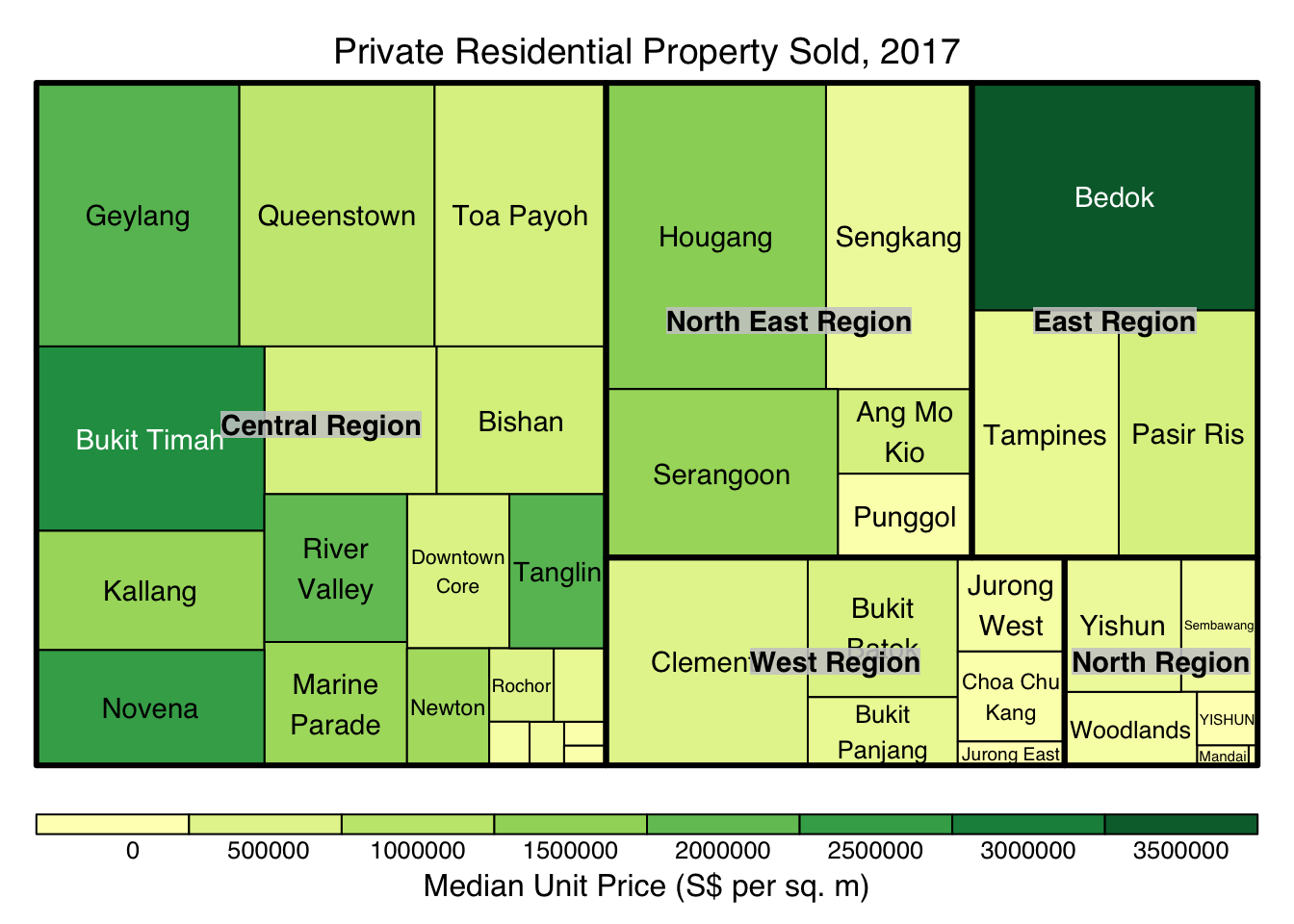
d3tree() is used to build and interactive treemap.

d3tree(tm,rootname = "Singapore" )

7 Reflections

Treemaps are good to visualize the ratios of numbers matching each criteria. This is one of the more aesthetic visualizations, in my opinion. However, I haven’t used it much.